
-
Abstract:
This paper presents a comprehensive analysis of the photometric system of the University of Chinese Academy of Sciences 70 cm Telescope located at the Yan-qi Lake campus of the University of Chinese Academy of Sciences. We evaluated the linearity, bias stability, and dark current of the camera. Utilizing the Johnson-Cousins Blue-Visible-Red-Infrared filter system and an Andor DZ936 charge-coupled device camera, we conducted extensive observations of Landolt standard stars to determine the color terms, atmospheric extinction coefficients, photometric zero-points, and the sky background brightness. The results indicate that this telescope demonstrates excellent performance in photometric calibration and good system performance overall, meeting the requirements for limited scientific research and teaching purposes.
-
1. INTRODUCTION
Located at the University of Chinese Academy of Sciences, Yan-qi Lake, Huairou, Beijing, the UCAS 70 cm Telescope (UCASST) is a Corrected Dall-Kirkham (CDK) telescope manufactured by Planewave Instruments
1 . The coordinates of the site are 40°24ʹ34ʹʹN, 116°40ʹ35ʹʹE at an altitude of 96 m above sea level. UCASST is managed by the School of Astronomy and Space Science at the University of Chinese Academy of Sciences and has been in operation for 2 years.It is mainly used for student practice and research purposes. The main science activities conducted with UCASST in recent years concern cataclysmic variables (CVs), follow-up observations of supernovae (SNe), and studies on the occultation of Neptune's moon, Triton[1,2]. Major objectives performed by UCASST include the 50 Mpc Nearby Galaxies Survey, with the goal of long-term monitoring of nearby galaxies within 50 Mpc of Earth[3] to discover transient sources. Alongside the UCASST survey observations, we have also conducted follow-up observations of newly discovered transient sources.
UCASST has also been used for relatively simple tasks, which make good use of its observing time and are suitable for teaching. These tasks include investigating CVs. Each of these highly variable close binary systems consists of a white dwarf accreting material from a low-mass companion[4]. Their variability includes large or small outbursts, moderate periodic variations of hours, and fast variations on the order of seconds to kiloseconds[5]. Capturing their variability is crucial for understanding their basic properties, such as orbital periods and superhump periods, and for revealing their active and variable accretion processes. Although several time-domain sky surveys, such as All-Sky Automated Survey for Supernovae (ASAS-SN)[6] and Zwicky Transient Facility (ZTF)[7], have been ongoing, their sparse sampling intervals (typically spaced over several days) make dedicated monitoring an important objective. Consequently, we conducted a CV monitoring project using UCASST from 2022 to 2023, aiming to characterize some poorly known systems. The 70 cm aperture allows us to achieve a sufficient signal-to-noise ratio (SNR) in a single image to observe an object at magnitudes down to 15.5.
Despite accumulating a large amount of observational data, the comprehensive testing of UCASST is still incomplete. Here, we report observations of a large number of standard stars using a Blue-Visible-Red-Infrared (BVRI) filter system and an Andor DZ936 charge-coupled device (CCD) camera
2 , providing systematic photometric zero-points, color index coefficients, and other parameters of UCASST, as well as measuring atmospheric extinction coefficients and on-site sky brightness. Additionally, we conducted a performance test of the camera to find out the linearity, bias stability, and dark current of the CCD.The overall structure of the paper is as follows: basic parameters of the observation system and observations are introduced in Section 2, CCD test results are described in Section 3, photometric calibrations are presented in Section 4, the system performance of UCASST is presented in Section 5, the scientific results produced by UCASST are presented in Section 6, and the conclusions and discussions are presented in Section 7.
2. OBSERVATIONS
2.1 Observation System
UCASST is equipped with a CCD camera to fulfill observation requirements and will support spectrometry in the near future. The CDK optical system shows excellent optical quality. With a
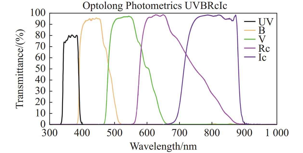
4557 mm focal length and F/6.5 focal ratio, the corrector enables a substantial 70 mm imaging circle. The UCASST filter system is equipped with seven filters, four of which are Johnson–Cousins BVRI filters3 ; the other three are Hα, [S II], and [O III] narrow-band filters. Fig. 1 shows the transmission curves for UBVRI filters. Center wavelengths and half-width wavelengths are presented in Table 1.![]() Figure 1. Transmission curves for the Johnson–Cousins UBVRI filters manufactured by Optolong.Table 1. Center wavelengths and half-width wavelengths of the Johnson–Cousins BVRI filters
Figure 1. Transmission curves for the Johnson–Cousins UBVRI filters manufactured by Optolong.Table 1. Center wavelengths and half-width wavelengths of the Johnson–Cousins BVRI filtersBand Name B V RCousins ICousins λc/nm 38.4 40.0 668.1 814.2 ∆λ/nm 0 40 180 160 In this work, all sources were observed using the Andor DZ936 CCD camera with the Johnson-Cousins BVRI filter system, the significant parameters of which are listed in Table 2 and Table 3. The combination of the telescope and the camera provides a resolution of 0.611ʹʹ pixel−1 with a 20.8ʹ × 20.8ʹ field of view (FoV).
Table 2. Parameters of the Andor DZ936 CCD cameraFeatures Specifications Pixel number 2048 ×2048 Pixel size 13.5 μm × 13.5 μm Imaging area 27.6 mm × 27.6 mm AD conversion 16 Bit Scan rates 50 kHz, 1 MHz, 3 MHz, 5 MHz Read noise @ 1MHz 6.4 e− Software-selectable gains 1×, 2×, 4× Gain @ 4x mode 1.0 e− /ADU Dark current 0.001 e−1 pix−1 s−1@ −70°C Nonlinearity <1% Table 3. Main parameters of the Planewave CDK700 observatory systemFeatures Specifications Optical design Corrected Dall-Kirkham Focal length 4557 mmAperture 700 mm Focal ratio F/6.5 Image circle 70 mm Image scale 22 μm/('') Focus port Two Nasmyth focus ports Mount type Alt/Az Motors Direct drive motors with encoders Maximum speed 10°/s 2.2 Observations
We performed photometry on Landolt standard stars from September 30, 2023, to June 4, 2024. The observed stars[8] are listed in Table 4. and the observation logs are given in Table 5. Here we should note that we generated Table 4. by cross-matching the observed standard stars with the Landolt catalog and extracting the matched items from the catalog. The complete Landolt catalog can be obtained through the Vizier website
4 . Table 5 includes the names of the observed standard stars, observation bands, exposure times, and the number of images taken for each band. We switched the filter after each exposure to ensure that the observation conditions for each band were as similar as possible.Table 4. Landolt's standard stars used for photometric calibrationStar α(J2000) δ(J2000) Vmag Bmag−Vmag Vmag−Rmag Rmag−Imag SA 92250 00 54 37 +00 38 56 13.178 0.814 0.446 0.394 SA 92253 00 54 52 +00 40 20 14.085 1.131 0.719 0.616 SA 92347 00 55 26 +00 50 49 15.752 0.543 0.339 0.318 SA 92348 00 55 30 +00 44 34 12.109 0.598 0.345 0.341 SA 93317 01 54 38 +00 43 00 11.546 0.488 0.293 0.298 SA 94171 02 53 38 +00 17 19 12.659 0.81 0.480 0.483 SA 94242 02 57 21 +00 18 38 11.728 0.301 0.178 0.184 SA 94296 02 55 20 +00 28 14 12.255 0.750 0.415 0.387 SA 94394 02 56 14 +00 35 10 12.273 0.545 0.344 0.330 SA 94401 02 56 31 +00 40 05 14.293 0.63 0.389 0.369 SA 94702 02 58 13 +01 10 53 11.594 1.418 0.756 0.673 SA 9515 03 52 40 −00 05 22 11.302 0.712 0.424 0.385 SA 9566 03 55 07 −00 09 31 12.892 0.715 0.426 0.438 SA 104461 12 43 07 −00 32 21 9.705 0.476 0.289 0.290 SA 113167 21 42 41 +00 16 08 14.841 −0.034 0.351 0.376 SA 114548 22 41 37 +00 59 07 11.601 1.362 0.738 0.651 PG0231+051 02 33 41 +05 18 40 16.105 −0.329 −0.16 −0.371 PG2213−006 22 16 28 −00 21 15 14.124 −0.217 −0.092 −0.110 Table 5. Observation log table of stars from the Landolt catalogObservation Date (yyyy/mm/dd) Target Band Exposure
time/sFrames
per band
2023/11/11SA 113167 B, V, R, I 10 54 SA 114548 B, V, R, I 10 10 PG0231+051 B, V, R, I 10 28 PG2213−006 B, V, R, I 10 45 2023/11/12 SA 92253 B, V, R, I 10 12 PG0231+051 B, V, R, I 10 23 2023/11/16 PG0231+051 B, V, R, I 30 30 2023/11/17 SA 93317 B, V, R, I 30 18 PG0231+051 B, V, R, I 30 12 2023/11/18 SA 92348 B, V, R, I 30 30 SA 93317 B, V, R, I 30 30 2023/11/19 SA 94171 B, V, R, I 30 29 SA 94296 B, V, R, I 30 29 SA 94394 B, V, R, I 30 16 2023/11/23 SA 94242 B, V, R, I 30 24 SA 94401 B, V, R, I 30 29 2023/11/24 SA 9515 B, V, R, I 30 33 SA 94401 B, V, R, I 30 30 2023/11/25 SA 95301 B, V, R, I 10 21 2023/12/01 SA 94401 B, V, R, I 30 30 SA 94702 B, V, R, I 30 13 2023/12/02 SA 94242 B, V, R, I 30 30 SA 9515 B, V, R, I 30 54 2023/12/03 SA 92250 B, V, R, I 30 20 SA 94242 B, V, R, I 30 27 SA 9515 B, V, R, I 30 23 2023/12/04 SA 92347 B, V, R, I 30 68 SA 9566 B, V, R, I 30 32 2024/05/30 SA 104461 B, V, R, I 10 18 Several cloudless, moonless photometric nights with good air quality were chosen during the target time period to perform accurate flux calibrations for UCASST using observed standard star data. Additionally, we determined the atmospheric extinction coefficient of the site by observing some star fields. For CCD testing, bias images were taken from June 6–8, 2024, for more than 30 hours, to test the bias stability. Tests for gain and readout noise used conventional observational data, and dome flat images were taken on June 16, 2024, to test the linearity.
3. CCD CALIBRATIONS
3.1 Bias
CCD bias refers to the baseline or offset voltage level present in each pixel of a CCD sensor during image capture. Bias is dependent on the characteristics of the CCD is being used, and by taking bias images with a 0-second exposure (i.e., direct readout with no exposure). By subtracting this biased image during image processing, we can correct the errors caused by the CCD bias. Bias stability has a significant impact on photometric accuracy.
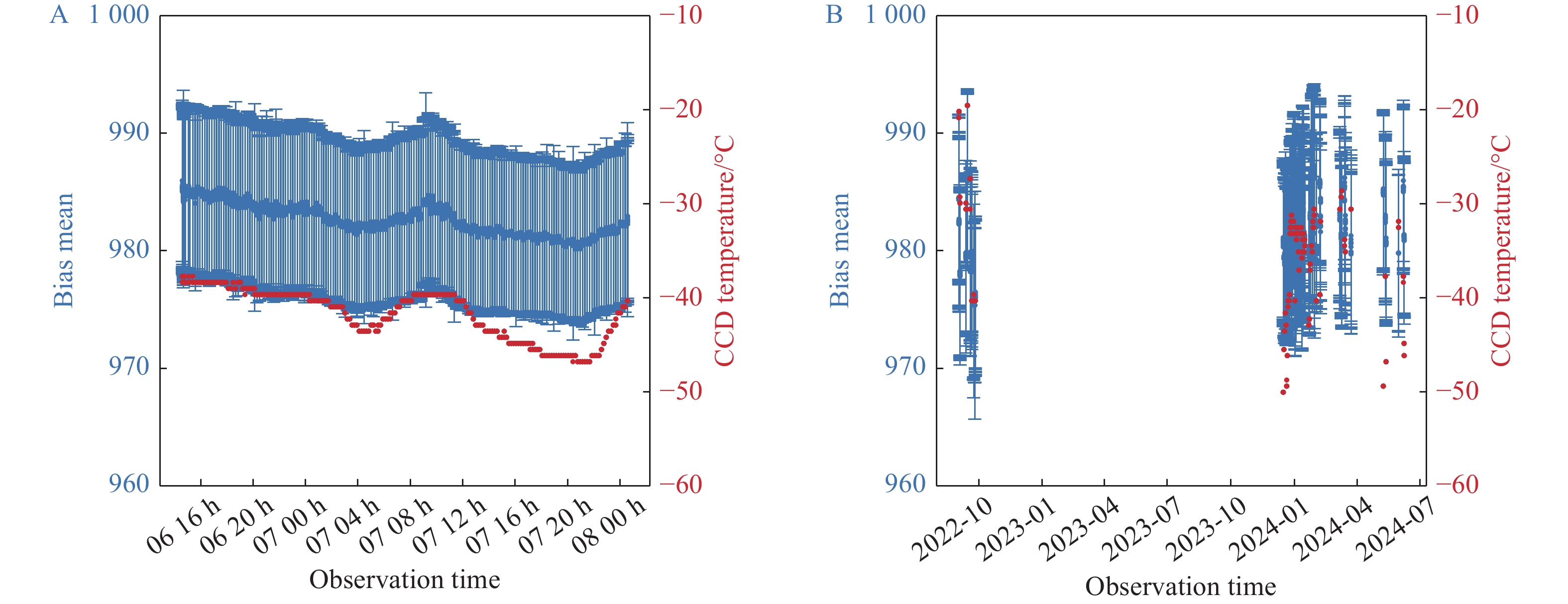
To test the bias stability, bias images were taken over 30 hours, with the results shown in Fig. 2A. We took 10 individual bias images with an exposure time of 0 s as a “bias group” for each observation, with a time interval of 10 minutes between each bias group.
![]() Figure 2. Stability test results on the bias of the Andor DZ936 CCD camera.The bias stability test results over 30 consecutive hours are shown in (A), and the long-term stability during over 20 months are shown in (B). The mean values and standard errors of these bias groups are shown as blue points with error bars, while the CCD temperature is shown with red dots.
Figure 2. Stability test results on the bias of the Andor DZ936 CCD camera.The bias stability test results over 30 consecutive hours are shown in (A), and the long-term stability during over 20 months are shown in (B). The mean values and standard errors of these bias groups are shown as blue points with error bars, while the CCD temperature is shown with red dots.For the long timespan bias test, bias data taken between September 2022 and June 2024 are shown in Fig. 2B. Similarly to the previous method, the bias group here was composed of bias images all recorded on the same day, providing a single data point. On the basis of these data, we concluded that the bias was stable and correlated with the temperature of the CCD during the observations. For longer timespans, the mean value of the bias did not change by much. Therefore, a single master bias can be used over the whole night, without involving time-variable corrections. Here we should note that the CCD temperature was not constant because of instabilities in the power supply at the observation site. At constant temperature, it is likely that the change in the bias will decrease.
3.2 Gain and Readout Noise
The gain and the read noise of the Andor DZ936 camera were tested. CCD gain is a parameter that describes the conversion factor between the number of electrons recorded in each pixel and the corresponding analog-to-digital units (ADU) that the camera outputs.
It is typically measured in electrons per ADU (e−/ADU). Knowing this value helps to evaluate the performance of a CCD. CCD readout noise is the electronic noise introduced during the process of reading out the charge from each pixel and converting it to a digital signal, and is measured in electrons (e−).
To give the gain and readout noise, two bias frames and two flat frames are needed[9]. The basic formulas for calculating the gain (G) and readout noise (RN ) are:
G=¯F1−¯B1+¯F2−¯B2σ2F1−F2−σ2B1−B2 (1) and
RN=G(σB1−B2)√2, (2) where F1 and F2 are the mean values of two independent flat images, while B1 and B2 are the mean values of two independent bias images. σF1−F2 and σB1−B2 are the standard deviation of the difference image of two independent flat images and the standard deviation of the difference image of two independent bias images, respectively.
A few days of twilight flat fields with different exposure times were chosen to test the gain and readout noise. We used the 4x mode of the Andor DZ936 camera, with a readout speed of 1 MHz. Detailed specifications given by the manufacturer can be found in Table 3, and our test results are shown in Table 6.
Table 6. Test results for gain and readout noiseTest date Readout mode Readout noise/ (e−) Gain/ (e− /ADU) Average readout noise/(e−) Average gain /(e− /ADU) 2024/02/01 4x @ 1 MHz 4.098 ± 0.017 0.985 ± 0.004 4.322 ± 0.018 1.024 ± 0.004 2024/03/09 4x @ 1 MHz 4.354 ± 0.018 1.043 ± 0.004 2024/03/13 4x @ 1 MHz 4.344 ± 0.018 1.003 ± 0.004 2024/03/22 4x @ 1 MHz 4.444 ± 0.019 1.044 ± 0.004 2024/05/11 4x @ 1 MHz 4.534 ± 0.019 1.039 ± 0.004 2024/05/12 4x @ 1 MHz 4.157 ± 0.017 1.029 ± 0.004 We found that the readout noise and the gain were stable over a long period of operation. The values of readout noise were comparatively lower than the corresponding values given by the manufacturer, and the gain values were similar to the corresponding value given by the manufacturer.
3.3 Linearity
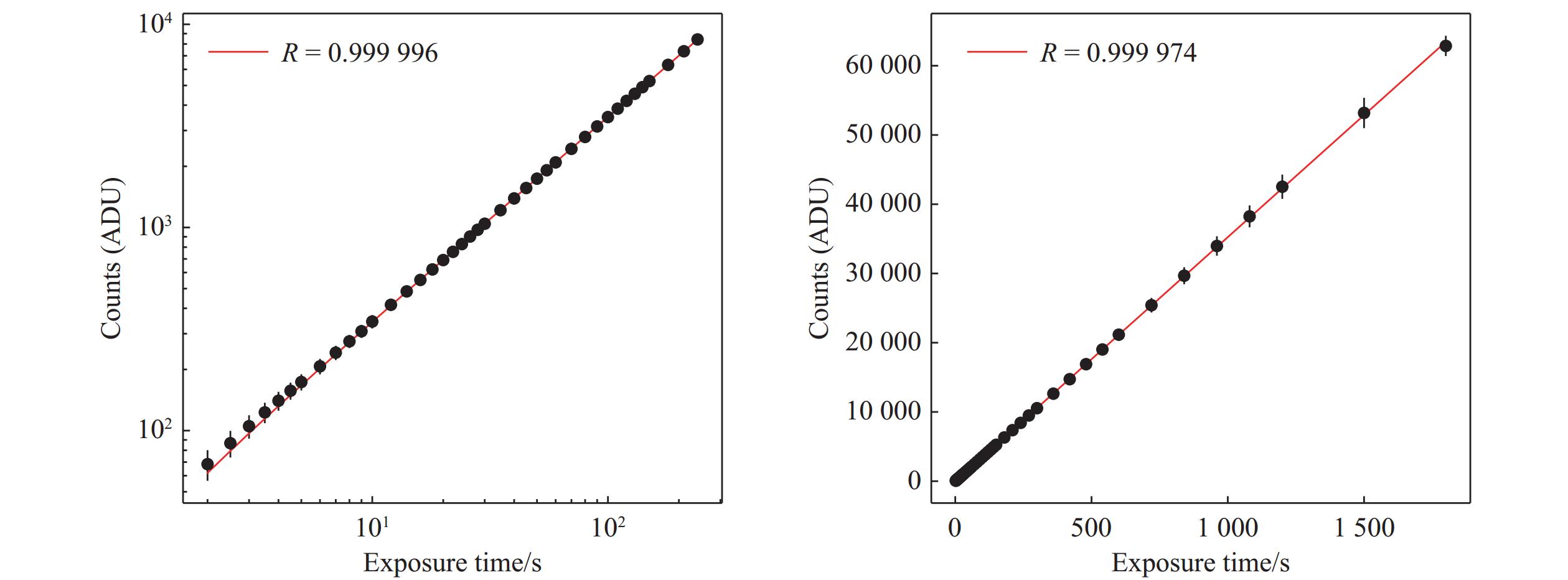
To test the linearity of the CCD camera, a stable in-dome light source was used to measure the ADU counts as a function of exposure time. We took these linearity test data in 4x mode at night on June 16, 2024, with the exposure times ranging from 2.0 s to
1800 s. Linearity test results are shown in Fig. 3. When the ADU count value was below10000 , the Andor DZ936 camera exhibited excellent linearity with a correlation coefficient of0.999996 . Over the entire range of the ADU count value up to60000 , the camera still kept perfect linearity, with a correlation coefficient of0.999974 .![]() Figure 3. Linearity test results of the Andor DZ936 camera. The correlation coefficients are
Figure 3. Linearity test results of the Andor DZ936 camera. The correlation coefficients are0.999 996 and0.999 974 for ADU counts up to10 000 and counts over the entire interval, respectively.3.4 Dark Current
Dark current is usually generated by the accumulation of electrons in the potential well of each pixel, and is expressed as the number of thermal electrons generated per second per pixel (e− pix−1 s−1). These signals, generated by thermal electrons, are indiscernible from light photons but can be ignored if the generation rate is low enough. Dark frames in this work were obtained on September 19 and 20, 2022, with integration times of 60 s, 120 s, 180 s, 300 s, and 600 s. We measured that the mean generation rate of the Andor DZ936 camera at –40°C was 0.074 e− pix−1 s−1. This dark current is relatively low, so dark correction can be neglected for short exposure observations.
4. PHOTOMETRIC CALIBRATIONS
To convert between the instrumental magnitude obtained by UCASST and the standard magnitude found in Landolt or other BVRI catalogs, precise photometric calibration is needed. Transform equations of a photometric calibration can be expressed as:
b=Bmag+ZB+k′BX+CB(Bmag−Vmag), (3) v=Vmag+ZV+k′VX+CV(Vmag−Rmag), (4) r=Rmag+ZR+k′RX+CR(Vmag−Rmag), (5) and
i=Imag+ZI+k′IX+CI(Rmag−Imag), (6) where b, v, r, and i are the instrumental magnitudes normalized to the exposure time of 1s, Bmag, Vmag, Rmag, and Imag are the standard magnitudes obtained by Landolt[8], ZB, ZV, ZR, and ZI are the zero-point magnitudes of the transformation, k'B, k'V, k'R, and k'I are the first-order atmospheric extinction coefficients, X is the airmass, CB, CV, CR, and CI are the color terms, and Bmag – Vmag, Vmag – Rmag, and Rmag – Imag are the color indices of the standard stars.
Here, photometry was performed using the sep
5 package, based on Python. The main photometric processes include bias combination, flat combination, CCD processing, World Coordinate System solving, background subtraction, and aperture photometry.4.1 Color Terms
By observing bright Landolt standard star fields or open clusters, we can determine the color terms for the transformations[10]. When calculating these two parameters, different stars in the same FoV were used, so their airmasses can be considered to be the same. This allows Equations (3)–(6) to be rewritten as:
b=Bmag+ZB+CB(Bmag−Vmag)+constant, (7) v=Vmag+ZV+CV(Vmag−Rmag)+constant, (8) r=Rmag+ZR+CR(Vmag−Rmag)+constant, (9) and
i=Imag+ZI+CI(Rmag−Imag)+constant. (10) From these equations, we can easily include different stars in the same FoV, with varying colors, to determine the color terms. Measurement results using different star fields, taken on different days, are presented in Table 7. Color terms were calculated from single or multiple star fields using the linear fitting method from the curvefit function in the scipy Python package. For the multiple star fields, weighted averages were performed to obtain a relatively accurate result. The overall result is the average value of the results obtained from every single date.
Table 7. Measured color termsTest date Center field star CB ± σCB CV ± σCV CR ± σCR CI ± σCI 2023/11/11 SA 113167 0.239 ± 0.012 −0.151 ± 0.010 −0.071 ± 0.009 −0.334 ± 0.012 PG0231+051 − 0.075 ± 0.029 0.082 ± 0.033 − PG2213−006 0.202 ± 0.006 −0.045 ± 0.007 0.042 ± 0.008 −0.197 ± 0.012 Weighted Average 0.209 ± 0.005 −0.071 ± 0.005 −0.004 ± 0.006 −0.265 ± 0.008 2023/11/12 SA 92253 0.239 ± 0.005 0.117 ± 0.003 0.183 ± 0.002 0.015 ± 0.003 SA 92330 0.257 ± 0.015 −0.007 ± 0.007 0.114 ± 0.003 −0.054 ± 0.004 PG0231+051 0.211 ± 0.015 0.033 ± 0.007 0.108 ± 0.004 − Weighted Average 0.238 ± 0.005 0.083 ± 0.003 0.148 ± 0.002 −0.017 ± 0.002 2023/11/16 PG0231+051 0.453 ± 0.008 −0.009 ± 0.006 0.107 ± 0.003 −0.100 ± 0.006 2023/11/17 PG0231+051 0.132 ± 0.018 0.008 ± 0.012 0.116 ± 0.007 −0.054 ± 0.007 2023/11/25 SA 95102 − − 0.074 ± 0.006 −0.256 ± 0.011 SA 95301 − −0.006 ± 0.006 0.058 ± 0.004 −0.065 ± 0.006 Weighted Average − −0.006 ± 0.006 0.064 ± 0.003 −0.109 ± 0.005 2023/12/02 SA 9515 0.151 ± 0.001 −0.046 ± 0.001 0.025 ± 0.001 −0.161 ± 0.001 2023/12/03 SA 9515 0.187 ± 0.002 −0.004 ± 0.002 0.023 ± 0.002 −0.167 ± 0.002 SA 92250 0.119 ± 0.011 −0.022 ± 0.006 0.069 ± 0.003 −0.106 ± 0.002 Weighted Average 0.184 ± 0.002 −0.006 ± 0.002 0.033 ± 0.001 −0.142 ± 0.002 2024/05/30 SA 104461 0.230 ± 0.020 0.071 ± 0.006 0.083 ± 0.003 −0.131 ± 0.005 Overall Average 0.228 ± 0.008 0.003 ± 0.005 0.072 ± 0.003 −0.122 ± 0.005 4.2 Atmospheric Extinction Coefficient
The atmospheric extinction coefficient is an important parameter for measuring atmospheric conditions at an observation site, and by measuring it with different filters, we are able to obtain the atmospheric extinction coefficients of different bands[11]. Because we are only concerned with the variation of one individual standard star with one airmass, the color term is held constant.
Here, Equations (3)–(6) can be rewritten as:
b=Bmag+ZB+k′BX+constant, (11) v=Vmag+ZV+k′VX+constant, (12) r=Rmag+ZR+k′RX+constant, (13) and
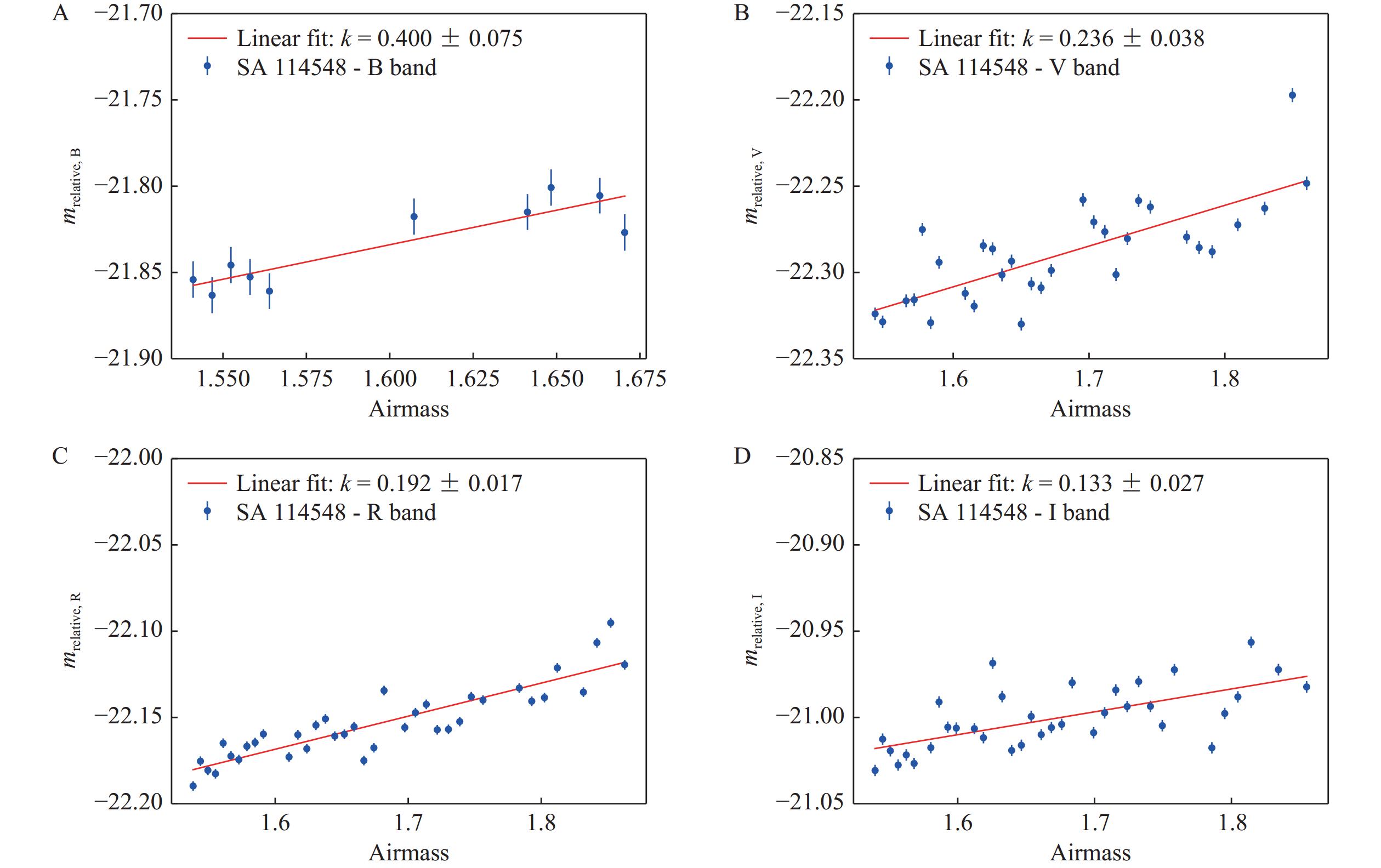
i=Imag+ZI+k′IX+constant, (14) where k'B, k'V, k'R, and k'I are the first-order atmospheric extinction coefficients. We assume that the atmospheric extinction coefficient k' does not change with time, so that it can be obtained easily using linear fitting. Fig. 4 gives an example of fitting the atmospheric extinction coefficient. The photometric data of SA 114 514 was observed on November 11, 2023, which was a clear and moonless photometric night. Several standard stars in the field were used to give the values of k' in different bands. Weighted averages were performed for different stars in the same band to give a relatively precise value of the k'. Final results are presented in Table 8.
![]() Figure 4. Images of atmospheric extinction coefficients obtained using Landolt standard stars in different bands. The x-axis shows airmass and the y-axis shows the difference between instrumental magnitude and standard magnitude presented in the Landolt catalog. The BVRI bands are plotted in (A), (B), (C), and (D).Table 8. Measured atmospheric extinction coefficients
Figure 4. Images of atmospheric extinction coefficients obtained using Landolt standard stars in different bands. The x-axis shows airmass and the y-axis shows the difference between instrumental magnitude and standard magnitude presented in the Landolt catalog. The BVRI bands are plotted in (A), (B), (C), and (D).Table 8. Measured atmospheric extinction coefficientsTest date k'B ± σk′B k'V ± σk′V k'R ± σk′R k'I ± σk′I 2023/11/11 0.322 ± 0.031 0.165 ± 0.018 0.156 ± 0.014 0.136 ± 0.018 2023/11/12 0.261 ± 0.022 0.177 ± 0.015 0.171 ± 0.011 0.079 ± 0.013 2023/11/16 0.320 ± 0.038 0.239 ± 0.016 0.145 ± 0.012 0.083 ± 0.021 2023/11/19 0.437 ± 0.051 0.288 ± 0.029 0.223 ± 0.021 0.168 ± 0.017 2023/11/23 0.314 ± 0.019 0.256 ± 0.019 0.181 ± 0.013 0.120 ± 0.018 2023/12/02 0.359 ± 0.015 0.286 ± 0.008 0.221 ± 0.008 0.151 ± 0.006 2024/05/30 − 0.114 ± 0.007 0.046 ± 0.006 0.012 ± 0.006 Overall average 0.336 ± 0.029 0.218 ± 0.016 0.163 ± 0.012 0.107 ± 0.014 Mu et al.[12] 0.335 ± 0.022 0.193 ± 0.018 0.090 ± 0.013 0.070 ± 0.017 4.3 Photometric Zero-points
After finding the values of color terms and atmospheric extinction coefficients, photometric zero-points of each band can be easily calculated using Equations (3)–(6). We used the mean value of the photometric zero-points of each star as the zero-point for a single image, and used the same method on each image as the zero-point for an entire photometric night.
In Table 9, we show photometric zero-points from different nights. The photometric zero-points show the effect of the observation environment and the instrument. For the photometric nights during November and December of 2023, the photometric zero-points were relatively stable. For the photometric observations on May 30, 2024, the zero-point was approximately 1.7 lower in each band, which indicated a change in the observing environment. We will further discuss this in Section 7.
Table 9. Measured photometric zero-pointsTest date ZB ± σZB ZV ± σZV ZR ± σZR ZI ± σZI 2023/11/11 −22.421 ± 0.161 −22.637 ± 0.090 −22.472 ± 0.079 −21.201 ± 0.083 2023/11/12 −22.387 ± 0.140 −22.632 ± 0.044 −22.433 ± 0.048 −21.108 ± 0.069 2023/11/16 −22.360 ± 0.301 −22.657 ± 0.011 −22.453 ± 0.066 −21.113 ± 0.057 2023/11/17 −22.380 ± 0.188 −22.636 ± 0.039 −22.436 ± 0.051 −21.233 ± 0.203 2023/11/18 −22.157 ± 0.148 −22.510 ± 0.066 −22.302 ± 0.045 −21.037 ± 0.052 2023/11/19 −22.174 ± 0.049 −22.479 ± 0.033 −22.249 ± 0.027 −21.017 ± 0.007 2023/11/23 −22.383 ± 0.156 −22.612 ± 0.048 −22.405 ± 0.023 −21.143 ± 0.047 2023/12/02 −22.361 ± 0.163 −22.552 ± 0.075 −22.367 ± 0.040 −21.065 ± 0.052 2024/05/30 −21.683 ± 0.146 −21.755 ± 0.053 −21.622 ± 0.038 −20.315 ± 0.074 4.4 Calibration Results
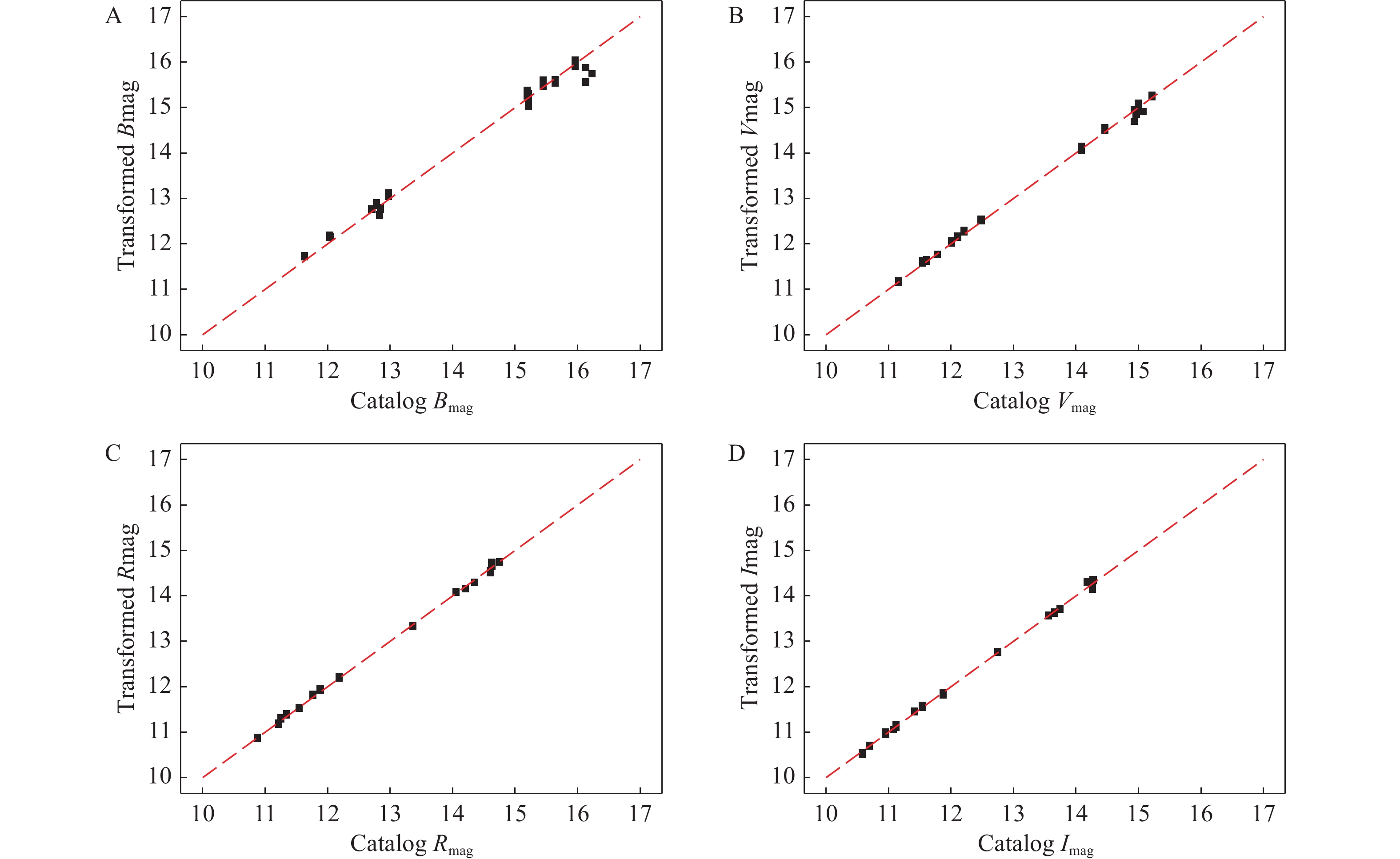
We used the data from November 18, 2023, for the photometric transformations and plotting, and results are shown in Fig. 5.
![]() Figure 5. Transformation fitting results for the BVRI bands. The data used for plotting was observed on November 18, 2023. The dotted red line shows the ideal transformation result, and the fitting slope from the data point is very close to 1.
Figure 5. Transformation fitting results for the BVRI bands. The data used for plotting was observed on November 18, 2023. The dotted red line shows the ideal transformation result, and the fitting slope from the data point is very close to 1.The standard deviations of the BVRI bands are 0.105, 0.040, 0.033, and 0.036, respectively. This means that we can make good transformations from instrumental magnitude to the standard Johnson–Cousins system. This can be performed using the equations:
b=(−22.157±0.148)+(0.336±0.029)X+(0.228±0.008)(Bmag−Vmag)+Bmag, σ=0.105, (15) v=(−22.510±0.066)+(0.218±0.016)X+(0.003±0.005)(Vmag−Rmag)+Vmag, σ=0.040, (16) r=(−22.302±0.045)+(0.163±0.012)X+(0.072±0.003)(Vmag−Rmag)+Rmag, σ=0.033, (17) and
i=(−21.037±0.052)+(0.107±0.014)X+(−0.122±0.005)(Rmag−Imag)+Imag, σ=0.036. (18) 5. SYSTEM PERFORMANCE
5.1 System Throughput
System throughput gives the overall efficiency, including the efficiency of optical components, transmission of the filters, quantum efficiency of the detector, and the transmission of the atmosphere[13]. The system throughput can be calculated as:
Eλ=Fλ10−0.4 mλπ(D2)2Δλ, (19) which finds the energy intake per second from a star of magnitude mλ in a circle of diameter D outside the Earth's atmosphere. Here, Fλ represents the flux of a 0-magnitude star at wavelength λ, and ∆λ represents the half-width of the transmission wavelength of the filter.
After finding Eλ , we can further calculate the incoming photons (Ncalc) as:
Ncalc=Eλhν=Eλλhc, (20) where h is the Planck constant and c is the speed of light. We can also calculate the extinction-corrected count rate of the CCD (Nobs ) as:
Nobs=Craw Texp 10−0.4kXG, (21) where Craw is the integrated count of the star, Texp is the exposure time, k is the first-order atmospheric extinction coefficient, X is the airmass, and G is the gain of the CCD. The total throughput E is defined as:
E=Nobs Ncalc . (22) Our calculation results are given in Table 10. Here we find a similar situation to the results of the photometric zero-points in Section 4.3, with the system throughput reaching its lowest on May 30, 2024.
Table 10. System throughput of different bandsDate System throughput/(%) B V R I 2023/11/11 11.26 11.89 7.15 2.46 2023/11/12 10.19 12.16 6.98 2.43 2023/11/16 11.57 13.02 7.38 2.58 2023/11/17 12.06 13.34 7.49 2.63 2023/11/18 8.81 11.33 6.62 2.44 2023/11/19 9.00 10.77 6.15 2.28 2023/11/23 9.70 12.26 6.95 2.57 2023/12/02 8.11 10.33 5.99 2.27 2024/05/30 4.82 5.57 3.29 1.12 5.2 Sky Background Brightness
Sky background brightness is a significant reference for performing observations. To estimate the sky brightness, we used the background functions in the photoutils Python package to extract and measure the flux of the sky background, which was transformed and normalized using Equations (3)–(6). The color terms and atmospheric extinction coefficients use the overall average values given in Table 7 and Table 8. Zero-points for each day can be found in Table 9.
The sky background brightnesses, measured on different days, are shown in Table 11, expressed in units of mag/arcsec2. The illumination of the Moon is shown in the last column, and the values in parentheses indicate the angle of the target from the Moon during the observation.
Table 11. Mean sky background brightnesses in various photometric bandsDate Mean sky background brightness/(mag/arcsec2) Moon illumination/(%) B V R I 2023/11/11 19.53 ± 0.24 18.67 ± 0.20 18.90 ± 0.18 19.31 ± 0.22 3.5 (Below horizon) 2023/11/12 19.97 ± 0.16 19.07 ± 0.16 19.16 ± 0.13 19.03 ± 0.14 1.0 (Below horizon) 2023/11/16 20.21 ± 0.03 19.40 ± 0.04 19.48 ± 0.04 19.09 ± 0.09 10.7 (Below horizon) 2023/11/17 19.75 ± 0.35 18.92 ± 0.26 19.11 ± 0.19 19.34 ± 0.09 18.5 (Below horizon) 2023/11/18 19.02 ± 0.11 18.13 ± 0.15 18.25 ± 0.16 18.90 ± 0.12 27.9 (58°) 2023/11/19 19.00 ± 0.22 18.14 ± 0.15 18.26 ± 0.14 18.78 ± 0.16 38.7 (33°) 2023/11/23 18.65 ± 0.06 17.90 ± 0.04 17.89 ± 0.07 17.74 ± 0.21 82.1 (34°) 2023/12/02 19.26 ± 0.16 18.36 ± 0.15 18.57 ± 0.13 19.06 ± 0.05 74.5 (78°) 2024/05/30 19.10 ± 0.04 18.06 ± 0.18 18.31 ± 0.18 18.38 ± 0.08 50.0 (Below horizon) On moonless photometric nights during November and December of 2023, the mean sky background brightness values of the BVRI bands were ~19.87 in the B band, ~19.02 in the V band, ~19.16 in the R band, and ~19.19 in the I band. During the moonless photometric night on May 30, 2024, the sky background brightness increased substantially, and significantly correlates with a drop in zero-point magnitude and system throughput. Comparisons with observations taken at the Yan-qi Lake Observatory and other professional observatories are shown in Table 12. We find that the night sky brightness at Yan-qi Lake is much higher than most other professional observatories, and compared with that in 2023, the night sky brightness in 2024 has significantly increased. We have subsequently communicated with the relevant departments of the Yan-qi Lake campus and made efforts to control light pollution near the observatory.
Table 12. Sky background brightnesses at different observatoriesObservatory Sky background brightness/(mag/arcsec2) Reference B V R I Xinglong 21.70 21.20 20.50 19.10 Shi et al.[14] 20.90 20.00 19.30 18.10 Huang et al. [10] Lulin 22.00 21.3 21.00 19.50 Kinoshita et al. [13] Weihai 20.17 18.90 18.95 19.11 Hu et al.[15] La Palma 22.70 21.90 21.00 20.00 Benn & Ellison[16] Paranal 22.60 21.60 20.90 19.70 Patat[17] Yan-qi Lake (2023) 19.87 19.02 19.16 19.19 this work Yan-qi Lake (2024) 19.10 18.06 18.31 18.38 this work 5.3 Limiting Magnitude and Photometric Precision
The SNR of an observed object[9] can be calculated as:
RSN=Nstar √Nstar +npix(NS+ND+N2R), (23) where Nstar is the total number of photons received from the source, NS, ND, and NR are the total number of photons given by the sky background, the dark current per pixel, and the CCD readout noise (in Section 3.2), respectively. npix is the whole pixel area used for the SNR calculation. Table 13 shows the limiting magnitudes of the different moonless photometric nights with corresponding exposure time when RSN = 10.
Table 13. Limiting magnitudes of BVRI bands measured on moonless photometric nightsDate Limiting magnitude/mag Exposure time/s B V R I 2023/11/11 15.54 15.57 15.60 15.19 10 2023/11/12 15.50 15.78 15.70 15.00 10 2024/05/30 14.94 14.70 15.16 14.50 10 2023/11/16 16.73 16.80 16.62 16.04 30 2023/11/17 16.31 16.23 16.24 16.20 30 The limiting magnitudes for RSN = 10, with an exposure time of 10 s in November 2023, are 15.5 in the B band, 15.7 in the V band, 15.6 in the R band, and 15.1 in the I band; they decrease to 14.9 in the B band, 14.7 in the V band, 15.2 in the R band, and 14.5 in the I band during May of 2024.
The limiting magnitudes at RSN = 10, with a 30 s exposure during November 2023, are 16.5 in the B band, 16.5 in the V band, 16.4 in the R band and 16.1 in the I band.
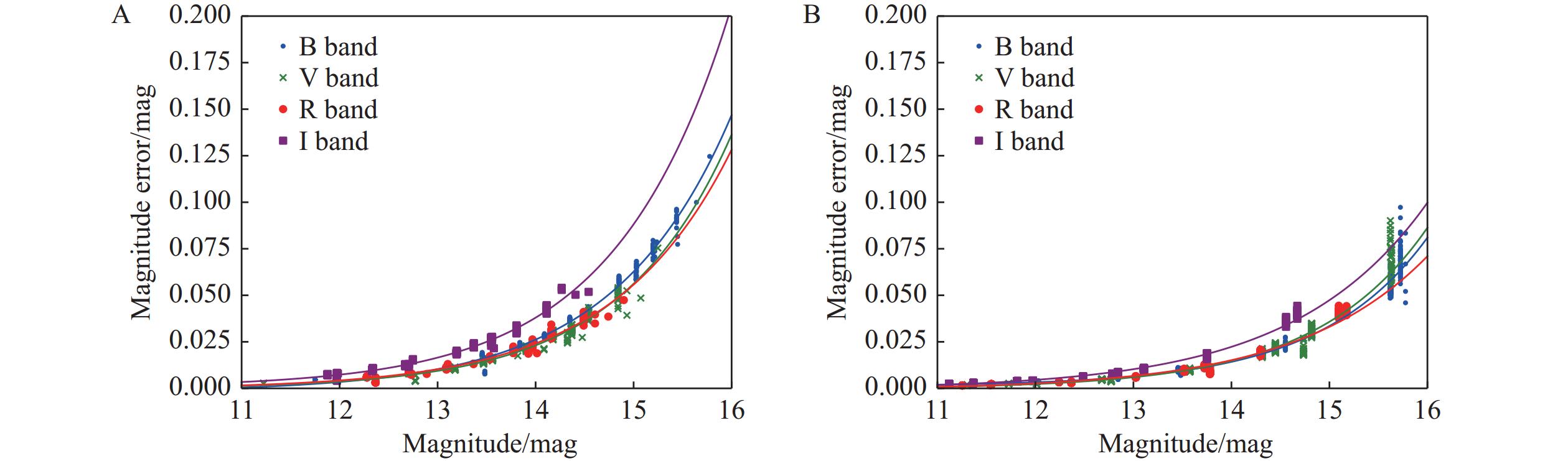
The errors of Landolt standard stars observed on moonless photometric nights are shown in Fig. 6. The photometric precision of a 30 s exposure is ≤0.01 mag for stars brighter than 13.6 in the B and V bands, 13.5 in the R band, and 13.0 in the I band. For an exposure time of 10 s, the corresponding values are 13.0 in the B, V, and R bands, and 12.4 in the I band.
![]() Figure 6. Magnitudes plotted against magnitude errors for moonless photometric nights.(A) the magnitudes against magnitude errors for a 10 s exposure time. (B) the same for a 30 s exposure time.
Figure 6. Magnitudes plotted against magnitude errors for moonless photometric nights.(A) the magnitudes against magnitude errors for a 10 s exposure time. (B) the same for a 30 s exposure time.6. RESULTS
Because UCASST has a relatively low limiting magnitude, it is well-suited to observing bright sources such as supernovae and bright variables. Taking this into consideration, we organized two different observing tasks on UCASST, including the Nearby Galaxies Survey and the Cataclysmic Variables Monitoring Program.
For the Nearby Galaxies Survey, UCASST is capable of performing both survey and follow-up observations of transient targets because of its medium-sized FoV. The observed targets are shown in Table 14, including nearby galaxies and supernovae.
Table 14. Targets observed by the Nearby Galaxies SurveyName R.A. Dec. Object Type Total
observations (Days)SN 2023bvj 09 : 50 : 56 +33 : 33 : 11 SN 20 SN 2023ixf 14 : 03 : 39 +54 : 18 : 42 SN 76 SN 2023wuk 22 : 19 : 30 +29 : 23 : 18 SN 7 SN 2023zqy 11 : 15 : 22 +31 : 31 : 25 SN 13 SN 2024gy 12 : 15 : 51 +13 : 06 : 56 SN 21 SN 2024jz 15 : 33 : 05 −01 : 37 : 30 SN 19 SN 2024ka 12 : 04 : 10 +01 : 49 : 34 SN 20 SN 2024ws 08 : 28 : 40 +73 : 44 : 53 SN 21 SN 2024any 03 : 08 : 57 −02 : 57 : 19 SN 10 SN 2024apt 10 : 25 : 37 −02 : 12 : 40 SN 12 SN 2024bch 10 : 21 : 48 +56 : 55 : 49 SN 11 M 61 12 : 21 : 55 +04 : 28 : 26 G 41 M 77 02 : 42 : 41 −00 : 00 : 48 G 34 M 81 09 : 55 : 33 +69 : 03 : 55 G 45 M 109 11 : 57 : 36 +53 : 22 : 28 G 37 NGC 2841 09 : 22 : 03 +50 : 58 : 35 G 33 NGC 6946 20 : 34 : 52 +60 : 09 : 13 G 28 We acquired and compiled these notable supernovae from the Transient Naming Server
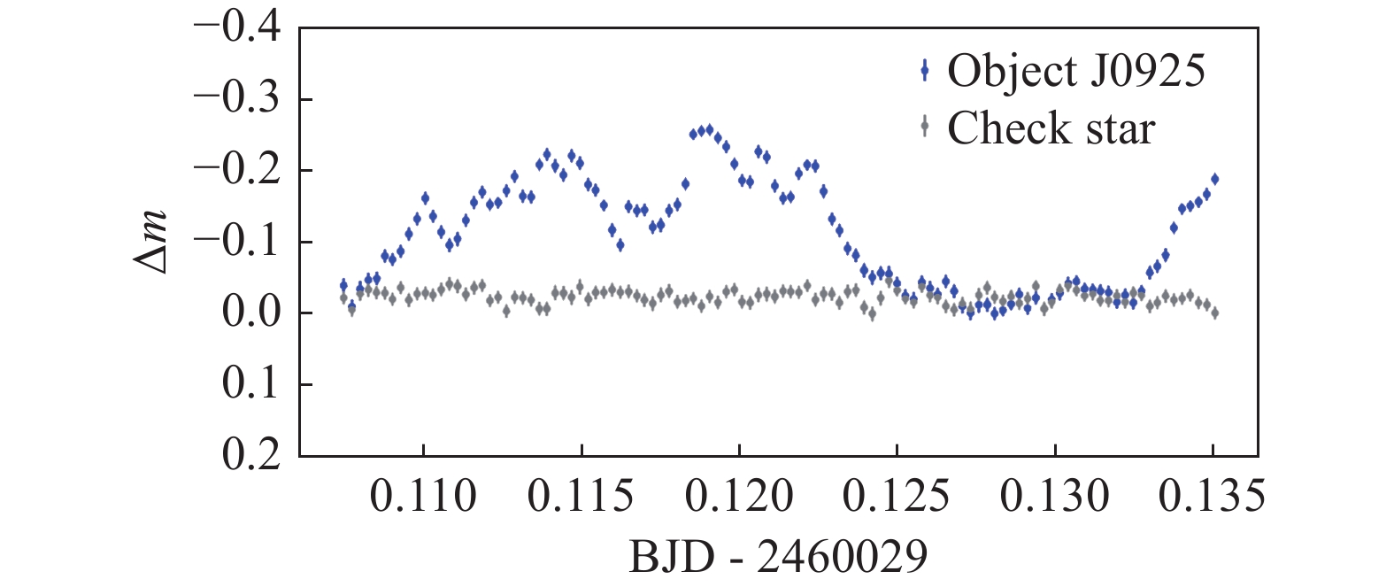
6 (TNS), and performed long-term observations. For the galaxies presented, we only concentrated on the relatively near and bright galaxies because of the low detection efficiency of UCASST.For the Cataclysmic Variables Monitoring Program, we selected two CVs observed by the Large Sky Area Multi-Object Fiber Spectroscopic Telescope (LAMOST) from Hou et al.[18] and Sun et al.[19] and a W Ursae Majoris-type eclipsing variable (EW-type) as observing targets. Specifically, we observed the bright (gmag = 13.3) nova-like star LAMOST J0925 (first reported by Hou et al.[18]) over seven nights using Johnson V or R filters with a 20 s exposure time.
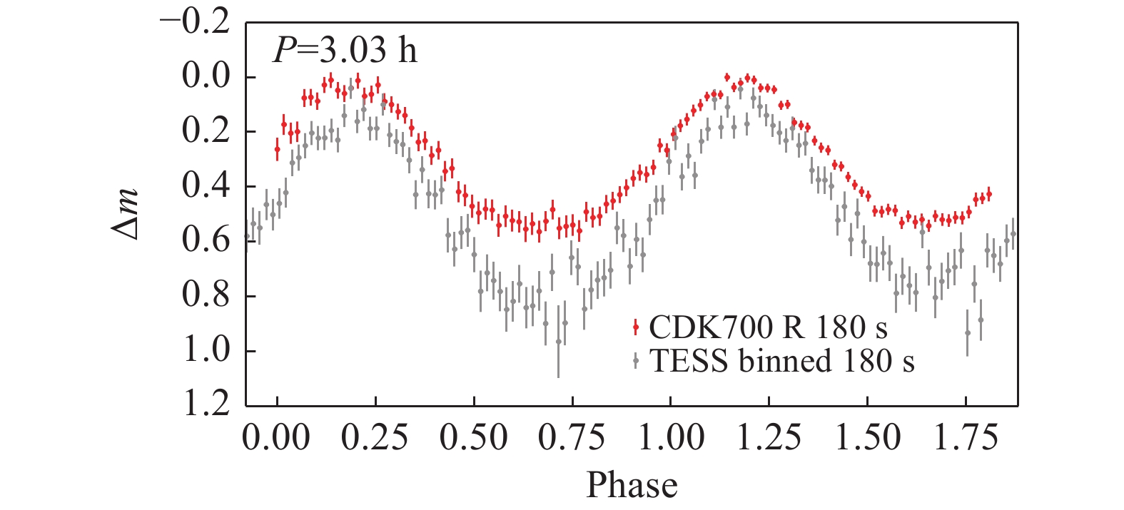
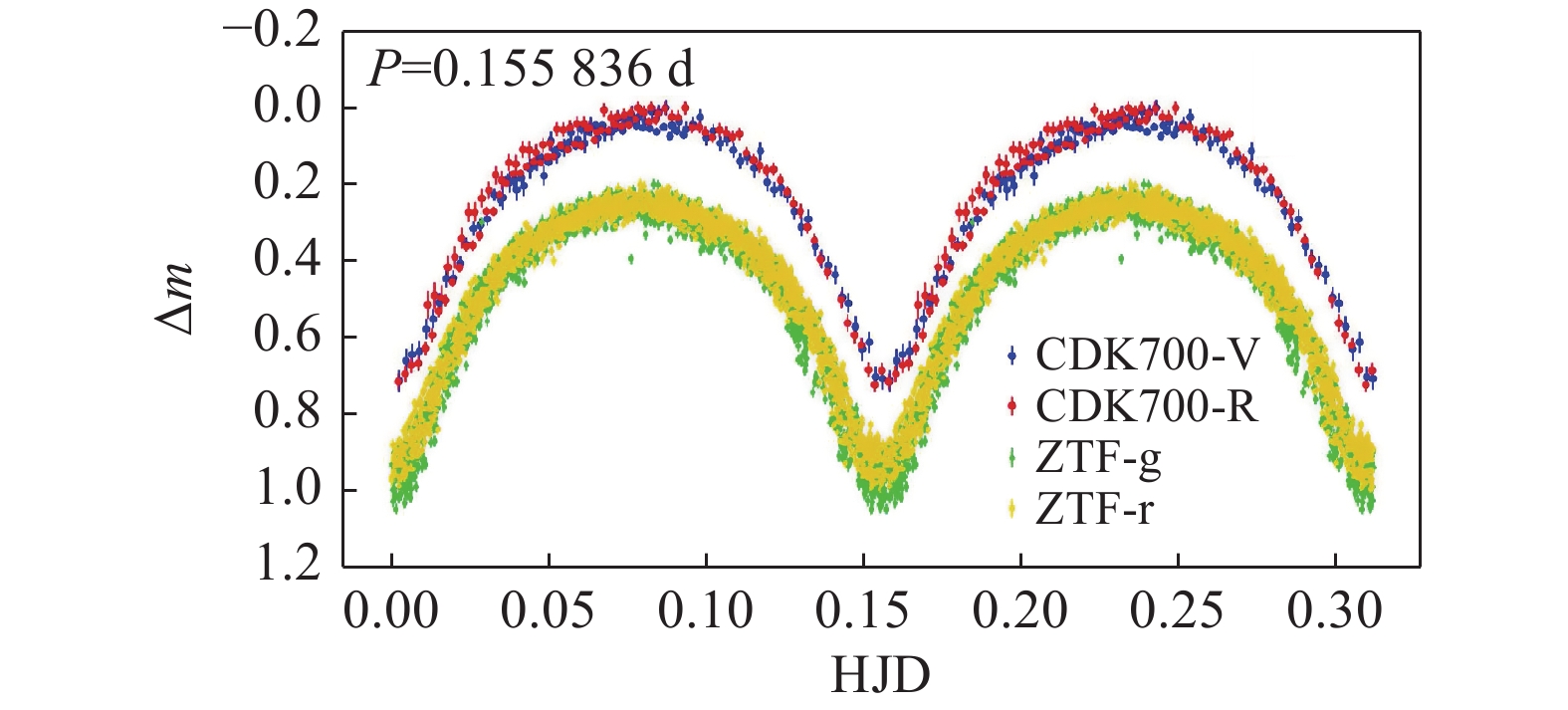
We performed differential photometry using circular apertures, and the resulting light curves clearly show significant rapid variations on a timescale of several minutes (see Fig. 7), which are likely due to accretion-induced flickering or quasi-periodic oscillations. The magnitude error of the target and the magnitude standard deviation of a nearby check star (which is approximately 0.06 mag fainter than the target) are both less than 0.01 mag. We also acquired light curves over 10 nights for the CV candidate LAMOST J0148 (gmag = 15.4, reported in Sun et al.[19]). The R band light curves give good results, compared with Transiting Exoplanet Survey Satellite (TESS) observations (see Fig. 8—note that the TESS fluxes are contaminated by a nearby source). The original 20-second cadence TESS light curve is binned to a 180-second cadence to match the 180-second exposure time of the UCASST observation. With a narrower filter bandwidth than that of TESS, UCASST achieves a higher SNR, demonstrating the ability of the telescope to observe relatively faint sources. Interestingly, there is an EW-type eclipsing variable star ATO J027+36 in the same FoV. The averaged V band magnitude of this variable is 15.49. In Fig. 9 we present the V and R band light curves of the EW-type variable, which are folded using a period of
0.155836 day, and compare them with the ZTF g and r band data. The real orbital period is twice this period. However, because the time coverage of the data is less than a single orbital period and the levels of the primary and secondary minimums differ slightly, we chose to fold the data by half the orbital period. The phase profiles obtained from UCASST observations and ZTF are consistent.7. DISCUSSION AND CONCLUSIONS
We have introduced UCASST and evaluated its photometric calibration, system performance, and basic site condition, finding that:
(1) Considering the basic parameters of the Andor DZ936 CCD camera, bias, gain, and readout noise of the CCD demonstrated good stability over short and long periods of time. The CCD has a good linearity up to approximately
60000 ADU and relatively low dark current for short exposure observations.(2) Deriving the coefficients of photometric calibrations based on Landolt standard stars, including color terms, first-order atmospheric extinction coefficients, and photometric zero-points, we found that the color terms are relatively small. This indicated that the BVRI system for UCASST has similar respond curves to the standard system used by Landolt.
The atmospheric extinction coefficients presented are stable, and the atmospheric extinction coefficients are slightly larger than those measured at Xinglong Observatory, which indicates good atmospheric conditions. Additionally, the photometric zero-points are stable during observation nights during November and December of 2023, and dropped 1.7 in each band on May 30, 2024 (see Table 9). This can be rationalized as being because of newly constructed street lights illuminating the telescope system during observations (see Fig. 10). This also explains the drop of system throughput, the elevated sky background brightness, and the decline in limiting magnitudes (see Tables 10, 11, and 13).
(3) The system performance of UCASST is evaluated in this work, including system throughput, limiting magnitude, photometric precision, and sky background brightness. The limiting magnitudes for UCASST, with RSN = 10 and a 30 s exposure time, are 16.5 in the B band, 16.5 in the V band, 16.4 in the R band, and 16.1 in the I band. The photometric precision for a 30 s exposure is ≤0.01 mag for stars brighter than 13.6 in the B and V bands, 13.5 in the R band, and 13.0 in the I band. The sky background brightness at the observation site is much higher than that of other professional observatories and continues to increase.
Because UCASST is located on the Yan-qi Lake campus of UCAS, the effect of the artificial lights is severe, which directly leads to limited observation depth and low SNR of observations. We strongly urge that the effects of artificial light in the vicinity of UCASST should be minimized during observation time so that UCASST can be used under the best possible observation conditions.
UCASST can be used for limited scientific research, such as studying bright binaries, observing nearby supernovae, monitoring CVs, and observing bright occultations. It is also well-suited to teaching purposes.
ACKNOWLEDGMENTS: This work was supported by National Key R&D Program of China (2023YFA1609700) and Research and Education Integration Funding. We thank for University of Chinese Academy of Sciences for providing the UCASST. -
![]()
Figure 1. Transmission curves for the Johnson–Cousins UBVRI filters manufactured by Optolong.
![]()
Figure 2. Stability test results on the bias of the Andor DZ936 CCD camera.
The bias stability test results over 30 consecutive hours are shown in (A), and the long-term stability during over 20 months are shown in (B). The mean values and standard errors of these bias groups are shown as blue points with error bars, while the CCD temperature is shown with red dots.
![]()
Figure 3. Linearity test results of the Andor DZ936 camera. The correlation coefficients are
0.999 996 and0.999 974 for ADU counts up to10 000 and counts over the entire interval, respectively.![]()
Figure 4. Images of atmospheric extinction coefficients obtained using Landolt standard stars in different bands. The x-axis shows airmass and the y-axis shows the difference between instrumental magnitude and standard magnitude presented in the Landolt catalog. The BVRI bands are plotted in (A), (B), (C), and (D).
![]()
Figure 5. Transformation fitting results for the BVRI bands. The data used for plotting was observed on November 18, 2023. The dotted red line shows the ideal transformation result, and the fitting slope from the data point is very close to 1.
![]()
Figure 6. Magnitudes plotted against magnitude errors for moonless photometric nights.
(A) the magnitudes against magnitude errors for a 10 s exposure time. (B) the same for a 30 s exposure time.
Table 1 Center wavelengths and half-width wavelengths of the Johnson–Cousins BVRI filters
Band Name B V RCousins ICousins λc/nm 38.4 40.0 668.1 814.2 ∆λ/nm 0 40 180 160  下载: 导出CSV
Table 2 Parameters of the Andor DZ936 CCD camera
Features Specifications Pixel number 2048 ×2048 Pixel size 13.5 μm × 13.5 μm Imaging area 27.6 mm × 27.6 mm AD conversion 16 Bit Scan rates 50 kHz, 1 MHz, 3 MHz, 5 MHz Read noise @ 1MHz 6.4 e− Software-selectable gains 1×, 2×, 4× Gain @ 4x mode 1.0 e− /ADU Dark current 0.001 e−1 pix−1 s−1@ −70°C Nonlinearity <1%
下载: 导出CSV
Table 3 Main parameters of the Planewave CDK700 observatory system
Features Specifications Optical design Corrected Dall-Kirkham Focal length 4557 mmAperture 700 mm Focal ratio F/6.5 Image circle 70 mm Image scale 22 μm/('') Focus port Two Nasmyth focus ports Mount type Alt/Az Motors Direct drive motors with encoders Maximum speed 10°/s
下载: 导出CSV
Table 4 Landolt's standard stars used for photometric calibration
Star α(J2000) δ(J2000) Vmag Bmag−Vmag Vmag−Rmag Rmag−Imag SA 92250 00 54 37 +00 38 56 13.178 0.814 0.446 0.394 SA 92253 00 54 52 +00 40 20 14.085 1.131 0.719 0.616 SA 92347 00 55 26 +00 50 49 15.752 0.543 0.339 0.318 SA 92348 00 55 30 +00 44 34 12.109 0.598 0.345 0.341 SA 93317 01 54 38 +00 43 00 11.546 0.488 0.293 0.298 SA 94171 02 53 38 +00 17 19 12.659 0.81 0.480 0.483 SA 94242 02 57 21 +00 18 38 11.728 0.301 0.178 0.184 SA 94296 02 55 20 +00 28 14 12.255 0.750 0.415 0.387 SA 94394 02 56 14 +00 35 10 12.273 0.545 0.344 0.330 SA 94401 02 56 31 +00 40 05 14.293 0.63 0.389 0.369 SA 94702 02 58 13 +01 10 53 11.594 1.418 0.756 0.673 SA 9515 03 52 40 −00 05 22 11.302 0.712 0.424 0.385 SA 9566 03 55 07 −00 09 31 12.892 0.715 0.426 0.438 SA 104461 12 43 07 −00 32 21 9.705 0.476 0.289 0.290 SA 113167 21 42 41 +00 16 08 14.841 −0.034 0.351 0.376 SA 114548 22 41 37 +00 59 07 11.601 1.362 0.738 0.651 PG0231+051 02 33 41 +05 18 40 16.105 −0.329 −0.16 −0.371 PG2213−006 22 16 28 −00 21 15 14.124 −0.217 −0.092 −0.110
下载: 导出CSV
Table 5 Observation log table of stars from the Landolt catalog
Observation Date (yyyy/mm/dd) Target Band Exposure
time/sFrames
per band
2023/11/11SA 113167 B, V, R, I 10 54 SA 114548 B, V, R, I 10 10 PG0231+051 B, V, R, I 10 28 PG2213−006 B, V, R, I 10 45 2023/11/12 SA 92253 B, V, R, I 10 12 PG0231+051 B, V, R, I 10 23 2023/11/16 PG0231+051 B, V, R, I 30 30 2023/11/17 SA 93317 B, V, R, I 30 18 PG0231+051 B, V, R, I 30 12 2023/11/18 SA 92348 B, V, R, I 30 30 SA 93317 B, V, R, I 30 30 2023/11/19 SA 94171 B, V, R, I 30 29 SA 94296 B, V, R, I 30 29 SA 94394 B, V, R, I 30 16 2023/11/23 SA 94242 B, V, R, I 30 24 SA 94401 B, V, R, I 30 29 2023/11/24 SA 9515 B, V, R, I 30 33 SA 94401 B, V, R, I 30 30 2023/11/25 SA 95301 B, V, R, I 10 21 2023/12/01 SA 94401 B, V, R, I 30 30 SA 94702 B, V, R, I 30 13 2023/12/02 SA 94242 B, V, R, I 30 30 SA 9515 B, V, R, I 30 54 2023/12/03 SA 92250 B, V, R, I 30 20 SA 94242 B, V, R, I 30 27 SA 9515 B, V, R, I 30 23 2023/12/04 SA 92347 B, V, R, I 30 68 SA 9566 B, V, R, I 30 32 2024/05/30 SA 104461 B, V, R, I 10 18
下载: 导出CSV
Table 6 Test results for gain and readout noise
Test date Readout mode Readout noise/ (e−) Gain/ (e− /ADU) Average readout noise/(e−) Average gain /(e− /ADU) 2024/02/01 4x @ 1 MHz 4.098 ± 0.017 0.985 ± 0.004 4.322 ± 0.018 1.024 ± 0.004 2024/03/09 4x @ 1 MHz 4.354 ± 0.018 1.043 ± 0.004 2024/03/13 4x @ 1 MHz 4.344 ± 0.018 1.003 ± 0.004 2024/03/22 4x @ 1 MHz 4.444 ± 0.019 1.044 ± 0.004 2024/05/11 4x @ 1 MHz 4.534 ± 0.019 1.039 ± 0.004 2024/05/12 4x @ 1 MHz 4.157 ± 0.017 1.029 ± 0.004
下载: 导出CSV
Table 7 Measured color terms
Test date Center field star CB ± σCB CV ± σCV CR ± σCR CI ± σCI 2023/11/11 SA 113167 0.239 ± 0.012 −0.151 ± 0.010 −0.071 ± 0.009 −0.334 ± 0.012 PG0231+051 − 0.075 ± 0.029 0.082 ± 0.033 − PG2213−006 0.202 ± 0.006 −0.045 ± 0.007 0.042 ± 0.008 −0.197 ± 0.012 Weighted Average 0.209 ± 0.005 −0.071 ± 0.005 −0.004 ± 0.006 −0.265 ± 0.008 2023/11/12 SA 92253 0.239 ± 0.005 0.117 ± 0.003 0.183 ± 0.002 0.015 ± 0.003 SA 92330 0.257 ± 0.015 −0.007 ± 0.007 0.114 ± 0.003 −0.054 ± 0.004 PG0231+051 0.211 ± 0.015 0.033 ± 0.007 0.108 ± 0.004 − Weighted Average 0.238 ± 0.005 0.083 ± 0.003 0.148 ± 0.002 −0.017 ± 0.002 2023/11/16 PG0231+051 0.453 ± 0.008 −0.009 ± 0.006 0.107 ± 0.003 −0.100 ± 0.006 2023/11/17 PG0231+051 0.132 ± 0.018 0.008 ± 0.012 0.116 ± 0.007 −0.054 ± 0.007 2023/11/25 SA 95102 − − 0.074 ± 0.006 −0.256 ± 0.011 SA 95301 − −0.006 ± 0.006 0.058 ± 0.004 −0.065 ± 0.006 Weighted Average − −0.006 ± 0.006 0.064 ± 0.003 −0.109 ± 0.005 2023/12/02 SA 9515 0.151 ± 0.001 −0.046 ± 0.001 0.025 ± 0.001 −0.161 ± 0.001 2023/12/03 SA 9515 0.187 ± 0.002 −0.004 ± 0.002 0.023 ± 0.002 −0.167 ± 0.002 SA 92250 0.119 ± 0.011 −0.022 ± 0.006 0.069 ± 0.003 −0.106 ± 0.002 Weighted Average 0.184 ± 0.002 −0.006 ± 0.002 0.033 ± 0.001 −0.142 ± 0.002 2024/05/30 SA 104461 0.230 ± 0.020 0.071 ± 0.006 0.083 ± 0.003 −0.131 ± 0.005 Overall Average 0.228 ± 0.008 0.003 ± 0.005 0.072 ± 0.003 −0.122 ± 0.005
下载: 导出CSV
Table 8 Measured atmospheric extinction coefficients
Test date k'B ± σk′B k'V ± σk′V k'R ± σk′R k'I ± σk′I 2023/11/11 0.322 ± 0.031 0.165 ± 0.018 0.156 ± 0.014 0.136 ± 0.018 2023/11/12 0.261 ± 0.022 0.177 ± 0.015 0.171 ± 0.011 0.079 ± 0.013 2023/11/16 0.320 ± 0.038 0.239 ± 0.016 0.145 ± 0.012 0.083 ± 0.021 2023/11/19 0.437 ± 0.051 0.288 ± 0.029 0.223 ± 0.021 0.168 ± 0.017 2023/11/23 0.314 ± 0.019 0.256 ± 0.019 0.181 ± 0.013 0.120 ± 0.018 2023/12/02 0.359 ± 0.015 0.286 ± 0.008 0.221 ± 0.008 0.151 ± 0.006 2024/05/30 − 0.114 ± 0.007 0.046 ± 0.006 0.012 ± 0.006 Overall average 0.336 ± 0.029 0.218 ± 0.016 0.163 ± 0.012 0.107 ± 0.014 Mu et al.[12] 0.335 ± 0.022 0.193 ± 0.018 0.090 ± 0.013 0.070 ± 0.017
下载: 导出CSV
Table 9 Measured photometric zero-points
Test date ZB ± σZB ZV ± σZV ZR ± σZR ZI ± σZI 2023/11/11 −22.421 ± 0.161 −22.637 ± 0.090 −22.472 ± 0.079 −21.201 ± 0.083 2023/11/12 −22.387 ± 0.140 −22.632 ± 0.044 −22.433 ± 0.048 −21.108 ± 0.069 2023/11/16 −22.360 ± 0.301 −22.657 ± 0.011 −22.453 ± 0.066 −21.113 ± 0.057 2023/11/17 −22.380 ± 0.188 −22.636 ± 0.039 −22.436 ± 0.051 −21.233 ± 0.203 2023/11/18 −22.157 ± 0.148 −22.510 ± 0.066 −22.302 ± 0.045 −21.037 ± 0.052 2023/11/19 −22.174 ± 0.049 −22.479 ± 0.033 −22.249 ± 0.027 −21.017 ± 0.007 2023/11/23 −22.383 ± 0.156 −22.612 ± 0.048 −22.405 ± 0.023 −21.143 ± 0.047 2023/12/02 −22.361 ± 0.163 −22.552 ± 0.075 −22.367 ± 0.040 −21.065 ± 0.052 2024/05/30 −21.683 ± 0.146 −21.755 ± 0.053 −21.622 ± 0.038 −20.315 ± 0.074
下载: 导出CSV
Table 10 System throughput of different bands
Date System throughput/(%) B V R I 2023/11/11 11.26 11.89 7.15 2.46 2023/11/12 10.19 12.16 6.98 2.43 2023/11/16 11.57 13.02 7.38 2.58 2023/11/17 12.06 13.34 7.49 2.63 2023/11/18 8.81 11.33 6.62 2.44 2023/11/19 9.00 10.77 6.15 2.28 2023/11/23 9.70 12.26 6.95 2.57 2023/12/02 8.11 10.33 5.99 2.27 2024/05/30 4.82 5.57 3.29 1.12
下载: 导出CSV
Table 11 Mean sky background brightnesses in various photometric bands
Date Mean sky background brightness/(mag/arcsec2) Moon illumination/(%) B V R I 2023/11/11 19.53 ± 0.24 18.67 ± 0.20 18.90 ± 0.18 19.31 ± 0.22 3.5 (Below horizon) 2023/11/12 19.97 ± 0.16 19.07 ± 0.16 19.16 ± 0.13 19.03 ± 0.14 1.0 (Below horizon) 2023/11/16 20.21 ± 0.03 19.40 ± 0.04 19.48 ± 0.04 19.09 ± 0.09 10.7 (Below horizon) 2023/11/17 19.75 ± 0.35 18.92 ± 0.26 19.11 ± 0.19 19.34 ± 0.09 18.5 (Below horizon) 2023/11/18 19.02 ± 0.11 18.13 ± 0.15 18.25 ± 0.16 18.90 ± 0.12 27.9 (58°) 2023/11/19 19.00 ± 0.22 18.14 ± 0.15 18.26 ± 0.14 18.78 ± 0.16 38.7 (33°) 2023/11/23 18.65 ± 0.06 17.90 ± 0.04 17.89 ± 0.07 17.74 ± 0.21 82.1 (34°) 2023/12/02 19.26 ± 0.16 18.36 ± 0.15 18.57 ± 0.13 19.06 ± 0.05 74.5 (78°) 2024/05/30 19.10 ± 0.04 18.06 ± 0.18 18.31 ± 0.18 18.38 ± 0.08 50.0 (Below horizon)
下载: 导出CSV
Table 12 Sky background brightnesses at different observatories
Observatory Sky background brightness/(mag/arcsec2) Reference B V R I Xinglong 21.70 21.20 20.50 19.10 Shi et al.[14] 20.90 20.00 19.30 18.10 Huang et al. [10] Lulin 22.00 21.3 21.00 19.50 Kinoshita et al. [13] Weihai 20.17 18.90 18.95 19.11 Hu et al.[15] La Palma 22.70 21.90 21.00 20.00 Benn & Ellison[16] Paranal 22.60 21.60 20.90 19.70 Patat[17] Yan-qi Lake (2023) 19.87 19.02 19.16 19.19 this work Yan-qi Lake (2024) 19.10 18.06 18.31 18.38 this work
下载: 导出CSV
Table 13 Limiting magnitudes of BVRI bands measured on moonless photometric nights
Date Limiting magnitude/mag Exposure time/s B V R I 2023/11/11 15.54 15.57 15.60 15.19 10 2023/11/12 15.50 15.78 15.70 15.00 10 2024/05/30 14.94 14.70 15.16 14.50 10 2023/11/16 16.73 16.80 16.62 16.04 30 2023/11/17 16.31 16.23 16.24 16.20 30
下载: 导出CSV
Table 14 Targets observed by the Nearby Galaxies Survey
Name R.A. Dec. Object Type Total
observations (Days)SN 2023bvj 09 : 50 : 56 +33 : 33 : 11 SN 20 SN 2023ixf 14 : 03 : 39 +54 : 18 : 42 SN 76 SN 2023wuk 22 : 19 : 30 +29 : 23 : 18 SN 7 SN 2023zqy 11 : 15 : 22 +31 : 31 : 25 SN 13 SN 2024gy 12 : 15 : 51 +13 : 06 : 56 SN 21 SN 2024jz 15 : 33 : 05 −01 : 37 : 30 SN 19 SN 2024ka 12 : 04 : 10 +01 : 49 : 34 SN 20 SN 2024ws 08 : 28 : 40 +73 : 44 : 53 SN 21 SN 2024any 03 : 08 : 57 −02 : 57 : 19 SN 10 SN 2024apt 10 : 25 : 37 −02 : 12 : 40 SN 12 SN 2024bch 10 : 21 : 48 +56 : 55 : 49 SN 11 M 61 12 : 21 : 55 +04 : 28 : 26 G 41 M 77 02 : 42 : 41 −00 : 00 : 48 G 34 M 81 09 : 55 : 33 +69 : 03 : 55 G 45 M 109 11 : 57 : 36 +53 : 22 : 28 G 37 NGC 2841 09 : 22 : 03 +50 : 58 : 35 G 33 NGC 6946 20 : 34 : 52 +60 : 09 : 13 G 28
下载: 导出CSV
-
[1] Sicardy, B., Tej, A., Gomes-Júnior, A. R., et al. 2024. Constraints on the evolution of the Triton atmosphere from occultations: 1989–2022. Astronomy & Astrophysics, 682: L24. doi: 10.1051/0004-6361/202348756
[2] Yuan, Y., Zhang, C., Li, F., et al. 2024. New constraints on Triton's atmosphere from the 6 October 2022 stellar occultation. Astronomy & Astrophysics, 684: L13. doi: 10.1051/0004-6361/202348460
[3] Ohlson, D., Seth, A. C., Gallo, E., et al. 2024. The 50 Mpc Galaxy Catalog (50 MGC): Consistent and homogeneous masses, distances, colors, and morphologies. The Astronomical Journal, 167(1): 31. doi: 10.3847/1538-3881/acf7bc
[4] Warner, B. 1995. Cataclysmic variable stars. Cambridge: Cambridge University Press.
[5] Warner, B. 2004. Rapid oscillations in cataclysmic variables. Publications of Astronomical Society of the Pacific, 116(816): 115−132.
[6] Shappee, B. J., Prieto, J. L., Grupe, D., et al. 2014. The man behind the curtain: X-rays drive the UV through NIR variability in the 2013 active galactic nucleus outburst in NGC 2617. The Astrophysical Journal, 788(1): 48. doi: 10.1088/0004-637X/788/1/48
[7] Bellm, E. C., Kulkarni, S. R., Graham, M. J., et al. 2019. The Zwicky Transient Facility: System overview, performance, and first results. Publications of Astronomical Society of the Pacific, 131(995): 018002. doi: 10.1088/1538-3873/aaecbe
[8] Landolt, A. U. 1992. UBVRI photometric standard stars in the magnitude range 11.5<V<16.0 around the celestial equator. The Astronomical Journal, 104: 340.
[9] Howell, S. B. 2000. Handbook of CCD Astronomy. Cambridge: Cambridge University Press.
[10] Huang, F., Li, J. Z., Wang, X. F., et al. 2012. The photometric system of the Tsinghua-NAOC 80-cm telescope at NAOC Xinglong Observatory. Research in Astronomy and Astrophysics, 12(11): 1585−1596.
[11] Zhou, A. Y., Jiang, X. J., Zhang, Y. P., et al. 2009. MiCPhot: A prime-focus multicolor CCD photometer on the 85-cm Telescope. Research in Astronomy and Astrophysics, 9(3): 349. doi: 10.1088/1674-4527/9/3/010
[12] Mu, H. Y., Fan, Z., Zhu, Y. N., et al. 2024. Astronomical test with CMOS on the 60 cm Telescope at the Xinglong Observatory, NAOC. Research in Astronomy and Astrophysics, 24(5): 055009. doi: 10.1088/1674-4527/ad359a
[13] Kinoshita, D., Chen, C. W., Lin, H. C., et al. 2005. Characteristics and performance of the CCD photometric system at Lulin Observatory. Chinese Journal of Astronomy and Astrophysics, 5(3): 315−326.
[14] Shi, H. M., Qiao, Q. Y., Hu, J. Y., et al. 1998. Characterization of the CCD system at the BAO 60 cm reflector for photometry. Acta Astrophysica Sinica, 18(1): 99−105. (in Chinese)
[15] Hu, S. M., Han, S. H., Guo, D. F., et al. 2014. The photometric system of the One-meter Telescope at Weihai Observatory of Shandong University. Research in Astronomy and Astrophysics, 14(6): 719. doi: 10.1088/1674-4527/14/6/010
[16] Benn, C. R., Ellison, S. L. 1999. La Palma night-sky brightness. arXiv: 9909153.
[17] Patat, F. 2003. UBVRI night sky brightness during sunspot maximum at ESO-Paranal. Astronomy & Astrophysics, 400(3): 1183−1198. doi: 10.1051/0004-6361:20030030
[18] Hou, W., Luo, A. L., Li, Y. B. et al. 2020. Spectroscopically identified cataclysmic variables from the LAMOST survey I. The sample. The Astronomical Journal, 159(2): 43. doi: 10.3847/1538-3881/ab5962
[19] Sun, Y. K., Cheng, Z. H., Ye, S., et al. 2021. A Catalog of 323 cataclysmic variables from LAMOST DR6. The Astrophysical Journal, Supplement Series, 257(2): 65. doi: 10.3847/1538-4365/ac283a
-
其他相关附件

计量
- 文章访问数: 176
- HTML全文浏览量: 10
- PDF下载量: 43
