1.   INTRODUCTION

Astronomical spectroscopic observations are an important part of modern astronomy, and by analyzing spectroscopic data from celestial objects, scientists can obtain key information about the chemical composition, physical properties, kinematic states, and the evolutionary history of their formation. Starting with the first detection of neutral hydrogen through the 21 cm line at 1420.4 MHz ^[1], the discovery of interstellar organic molecules was one of the four significant discoveries in astronomy in the 1960s, following the discovery of interstellar ammonia molecules by researchers in 1968^[2] and interstellar carbon monoxide molecules in the Orion Nebula in 1970^[3]. Observations of spectra have enabled astronomers to probe the molecular composition of the universe in different environments, especially in celestial bodies and celestial environments such as the interstellar medium, interstellar molecular clouds, planetary nebulae, and star-forming regions. Astronomical spectroscopy is an important tool for studying the chemical composition, physical properties, kinematics, and dynamics of objects in the universe. Spectroscopic observations can be used to study the kinematics and dynamics of objects and celestial environments in the universe^[4]; for example, observations of the strength and velocity of emission lines can be used to study the motions of the rotating arms of galaxies^[5], to study tidal motions of interacting galaxies, and to study turbulence and collapse in nebulae in star-forming regions^[6]. Observations can be used to trace the chemical composition and evolution of objects in their regions; for example, complex molecules are often formed on dust particles in cold, dense molecular clouds^[7]. Spectral observations can be used in astrophysical research. For example, the galactic plane survey of water masers can be used to study the relationship between maser distribution and star formation and evolution^[8]. Different critical densities of molecules reflect the gas density of their surrounding regions; for typical Ly α emitting galaxies, the hydrogen column density is α~10¹⁷–10²⁰ cm^−2[9].

The development of astronomical observation equipment and technology has brought about a surge in the amount of observation data, and the Large Sky Area Multi-Object Fiber Spectroscopic Telescope (LAMOST)^[10] is the multi-target spectroscopic telescope with the largest field of view and the highest spectral acquisition rate in the international astronomical community. The DR11 dataset released by LAMOST in September 2024 contains more than 10⁸ low- and medium-resolution spectra. Similarly, the Sloan Digital Sky Survey (SDSS)^[11] telescope generates approximately 10⁶ spectra per observation. The Anglo-Australian Telescope (AAT), a collaboration between the United Kingdom and Australia, uses a 2-degree field (2dF) multi-fiber spectrograph^[12] for its survey mission and has acquired spectra of more than one million objects. The Apache Point Observatory Galactic Evolution Experiment (APOGEE)^[13] is a high-resolution and high signal-to-noise near-infrared spectroscopic survey program, and the APOGEE DR12 dataset^[14] releases ~10⁵ red giant spectroscopic data. The rapid increase in data volume has placed considerable pressure on subsequent data preprocessing and scientific analysis processes. Spectral data preprocessing must go through background correction, skylight background removal, wavelength calibration, flux calibration, and continuum spectra fitting^[15,16]. Then, according to different scientific research objectives, the data are processed for classification, clustering, outlier analysis, and stellar atmospheric parameter measurements^[17]. Scientific research on spectral data relies on accurately extracting continuous spectral data and spectral line information in the preprocessing process^[18]. Traditional spectral data preprocessing and other processes rely on researchers using software such as IRAF^[19] to manually process the raw spectral data using an interactive approach, and the preprocessing steps need to be repeated for each spectral data file, which consumes a large amount of manual time and results in inefficient data processing.

By carrying out processing such as classification, clustering, outlier analysis, and stellar atmospheric parameter measurements on astronomical spectra, information can be deeply mined from massive data, which is of great significance for understanding the physical properties of celestial bodies, studying the chemical compositions of celestial bodies, investigating the state of celestial motion and discovering unknown celestial bodies. With the explosive growth of spectral data, the speed of spectral data mining has failed to develop synchronously, dramatically reducing the efficiency and scientific output of spectral data processing. However, the rise of artificial intelligence technology has provided a new solution to these difficulties.

Artificial intelligence is a technological science that studies and develops theories, methods, and application systems for modeling, extending, and expanding human intelligence, often implemented using machine learning (ML) methods. ML is a subfield of artificial intelligence that studies how to enable machines to simulate or implement human learning behaviors by learning to model from data through algorithms and statistical models. Deep-learning (DL) algorithms are ML methods based on artificial neural networks, which automatically extract features layer by layer from data by constructing multi-level neural networks. Commonly used DL algorithms include convolutional neural networks (CNNs), recurrent neural networks (RNNs), and generative adversarial networks (GANs).

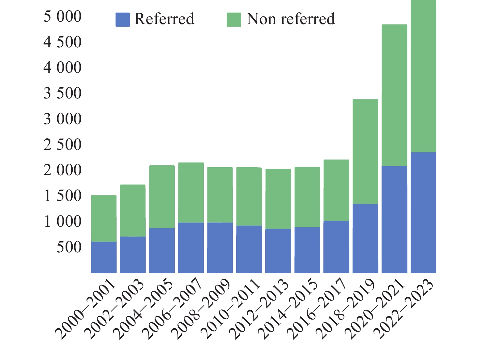
Computational methods were introduced to astronomy at the end of the 20th century, when simple algorithms were used to process telescope data, mainly for tasks such as orbit calculations and basic image processing. At the beginning of the 21st century, ML began to be widely used in astronomy, with algorithms such as neural networks, support vector machines, and multilayer perceptron machines being used to classify galaxies^[20], photometric redshift estimation^[21], and analyze cosmic microwave background data^[22]. According to the data retrieved from the Astrophysics Data System (ADS), the trend of growth in the number of papers containing the terms ML, DL, or deep neural network in their titles, abstracts, and keywords is depicted in Fig. 1, and the application of ML in astronomy has grown significantly after 2017.

Figure  1.  Number of papers with titles, abstracts, and keywords containing ML, DL, or deep neural network in the field of astronomy, 2000–2023.

下载: 全尺寸图片 幻灯片

2.   ML METHODS

2.1   Traditional ML Methods

Traditional ML methods include perceptron, k-nearest neighbors (kNN), decision trees, support vector machines (SVMs), clustering techniques, singular value decomposition (SVD), and principal component analysis (PCA). The perceptron is a fundamental linear classification model and one of the earliest forms of neural networks, which performs classification by learning a linear relationship between input features and target categories. The kNN method is an instance-based, nonparametric classification and regression approach. When classifying a sample, the kNN algorithm assigns a category based on the majority vote of its kNN in the feature space. Decision trees are a model that classifies data through a series of decision nodes, where each node represents a decision rule based on a feature, branches correspond to the outcomes of these rules, and leaf nodes represent the final classification. SVM is a supervised learning algorithm primarily used for classification and regression tasks. It separates data points by constructing a hyperplane that maximizes the margin between different classes, achieving optimal classification. Clustering refers to an unsupervised learning technique to partition a dataset into distinct groups or clusters, where data points within the same cluster are highly similar, and those in different clusters exhibit significant dissimilarity. SVD is a matrix factorization method that decomposes a matrix into the product of three matrices, including singular values and singular vectors. It is widely applied for dimensionality reduction, noise filtering, and data compression. PCA is a statistical technique used for dimensionality reduction, which transforms data into a new coordinate system by identifying the principal components that capture the most variance, reducing the number of variables while retaining essential information.

Traditional ML methods generally operate based on specific assumptions or rules, resulting in relatively low model computational complexity. However, the model training process heavily relies on data preprocessing, which requires domain experts to manually extract hand-crafted features from raw data. Traditional ML methods typically require smaller datasets and have relatively low computational resource demands. Most models exhibit good interpretability because their predictions can be easily understood by analyzing model parameters or decision rules. These models usually demonstrate good generalization ability on smaller datasets but often encounter performance bottlenecks when dealing with complex, large-scale data.

2.2   DL Methods

McCulloch and Pitts^[23] proposed the original artificial neural network model in 1943; Rosenblatt^[24] invented the perceptual machine in 1958, regarded as the predecessor of feedforward neural networks, Rumelhart et al.^[25] redeveloped the backpropagation algorithm for feedforward neural network learning in 1986, and Hinton et al.^[26] introduced the concept of DL in 2006, referring to ML that includes complex neural networks such as deep neural networks.

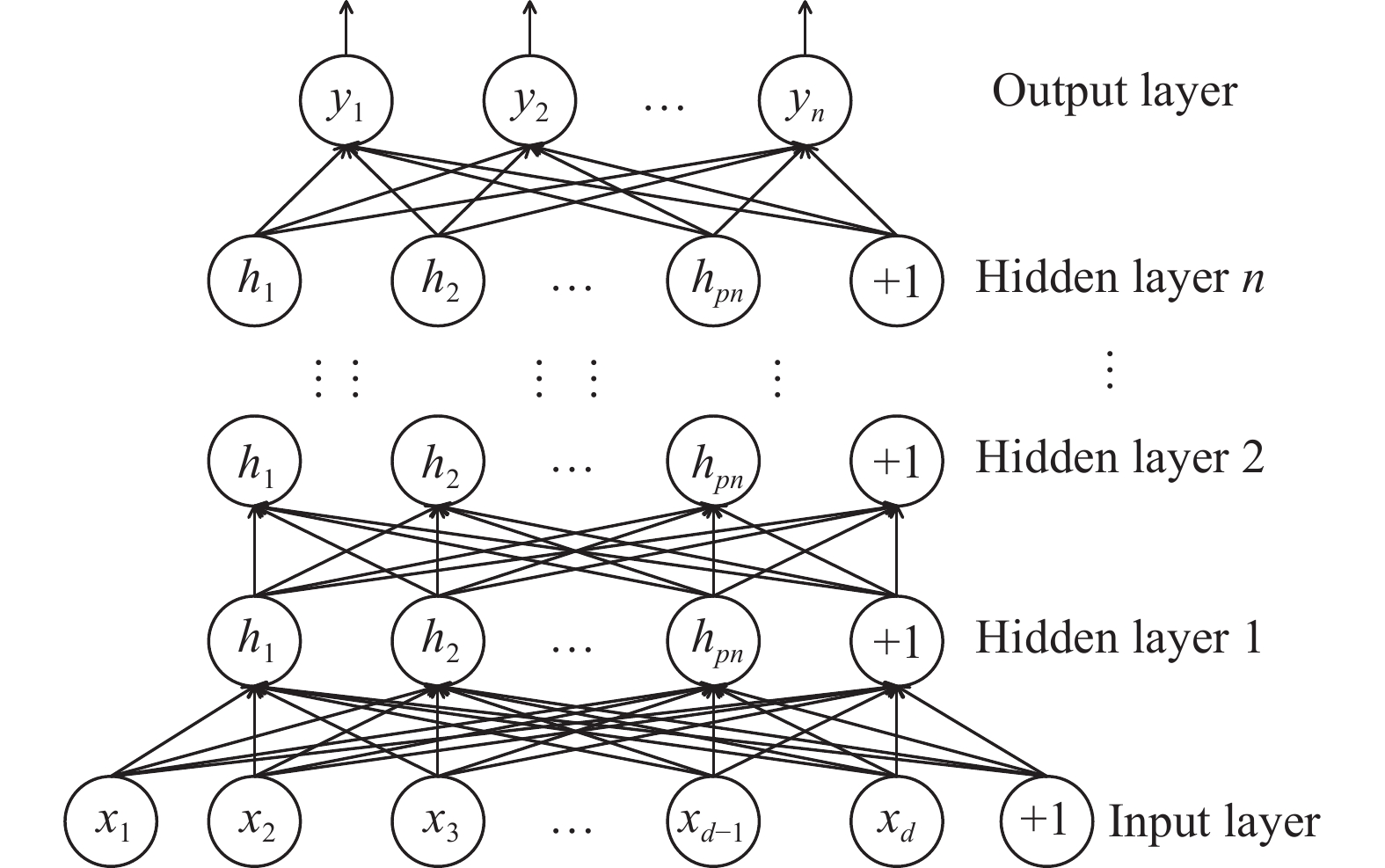
An artificial neural network is a network-like ML model composed of neuron connections inspired by biological neural networks. It was invented to mimic the structure of the human brain and its function as an information processing system. Artificial neural networks comprise an input layer, a hidden layer, and an output layer. Fig. 2 illustrates the structure of a deep neural network with n hidden layers; the input layer receives the input data, each input node corresponds to a feature of the data, the hidden layer contains multiple nodes, which process the input data through activation functions, the number and size of the hidden layers affects the network's complexity and learning ability, and the output layer is used to generate the final output results. The output layer generates the final output, such as category labeling in a classification task or numerical prediction in a regression task.

Figure  2.  Deep neural network structure with n hidden layers.

下载: 全尺寸图片 幻灯片

2.2.1   Feedforward Neural Networks

A feedforward neural network is the most representative neural network, composed of multiple layers of neurons, including an input layer, hidden layer, and output layer; the neurons between the layers are connected, the neurons within the layers are not connected, the output of the neurons of the former layer is the input of the neurons of the latter layer, and there is no feedback in the entire network, so the feedforward neural network cannot memorize. The input data are passed from the input layer to the output layer through the weighting and bias of each layer to produce the output result.

Artificial neural networks learn by adjusting the weights of the connections between neurons. The learning process is implemented through the backpropagation algorithm^[25], which calculates the loss function to evaluate the difference between the predicted and actual values and then updates the weights through optimization algorithms such as gradient descent to make the model gradually approach the optimal solution. Feedforward neural networks are used primarily in classification problems, regression problems, pattern recognition, and other tasks.

2.2.2   CNNs

A CNN is a neural network for predicting image data (grid-structured data) with a hierarchical grid structure, which can be regarded as a special feedforward neural network. The basic structure of a CNN consists of an input layer, a convolutional layer, a pooling layer, a fully-connected layer, and an output layer. The convolutional layer scans the input data through a convolutional kernel, automatically extracts the low-level features such as edges and textures, and then progressively extracts the high-level features through multilayer convolution; the pooling layer is used for downsampling to reduce the size of the feature maps and reduce the complexity of the computation while retaining the key information; the fully-connected layer maps the previously extracted features to the output. The fully-connected layer maps the previously extracted features to the output, such as the results of classification or regression tasks.

The application areas of CNNs include computer vision, natural language, and speech processing. They are used in computer vision for tasks such as image classification, target detection, and image segmentation, and they are the core models in this field. Fukushima^[27] proposed the Necocognitron model in 1980, and LeCun et al.^[28] proposed the LeNet-5 model in 1989 based on the inverse propagation algorithm to propose the LeNet-5 model; these models achieved good recognition results on small image recognition but poor recognition results on large-scale data^[29]. Then, in 2012, Krizhevsky et al.^[30] developed a CNN called AlexNet to obtain the best classification results to date in the ImageNet large-scale image classification challenge competition.

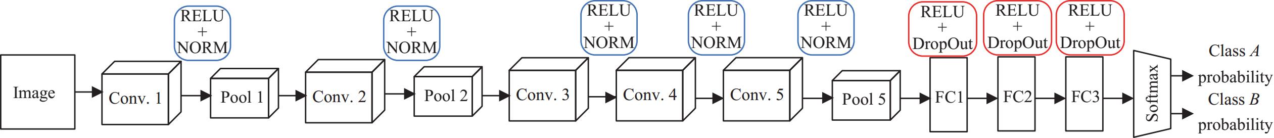
The power of CNNs in processing high-dimensional data such as images and signals makes it equally suitable for spectral analysis and data classification tasks in astronomy. Shi et al.^[31] designed SCNet network based on the CNN model used to classify stellar spectral images. The model was compared with many typical classification networks in DL to achieve the 0.861 highest classification accuracy; Aniyan et al.^[32] used CNN for radio galaxy classification, the model architecture is depicted in Fig. 3, the number of training samples, precision, recall, F₁ score, and test samples of the model are presented in Table 1, and the classification effect is comparable to the manual classification but much faster; Keown et al.^[33] used CNN for the multi-peak spectra fitting identification and classification, which was tested on 30000 datasets consisting of noisy, single-peak, and bimodal spectra, and the classification accuracies reached 100%, 99.92% ± 0.02%, and 96.72% ± 0.18%.

Figure  3.  CNN architecture for radio galaxy classification with output as probability scores for two galaxy classes^[32].

下载: 全尺寸图片 幻灯片

Table  1.  Class of the sources, size of the training samples for each class, precision, recall, and F₁ classification score for the validation sample and the support^[32]

Class	Training samples		Precision/(%)	Recall/(%)	F1 score/(%)	Support
	Actual	Augmented
Bent-tailed	177	25 488	95	79	87	77
FR I	125	36 000	91	91	91	53
FR II	227	32 688	75	91	83	57
Average			88	86	86	187

下载: 导出CSV 

| 显示表格

2.2.3   RNNs

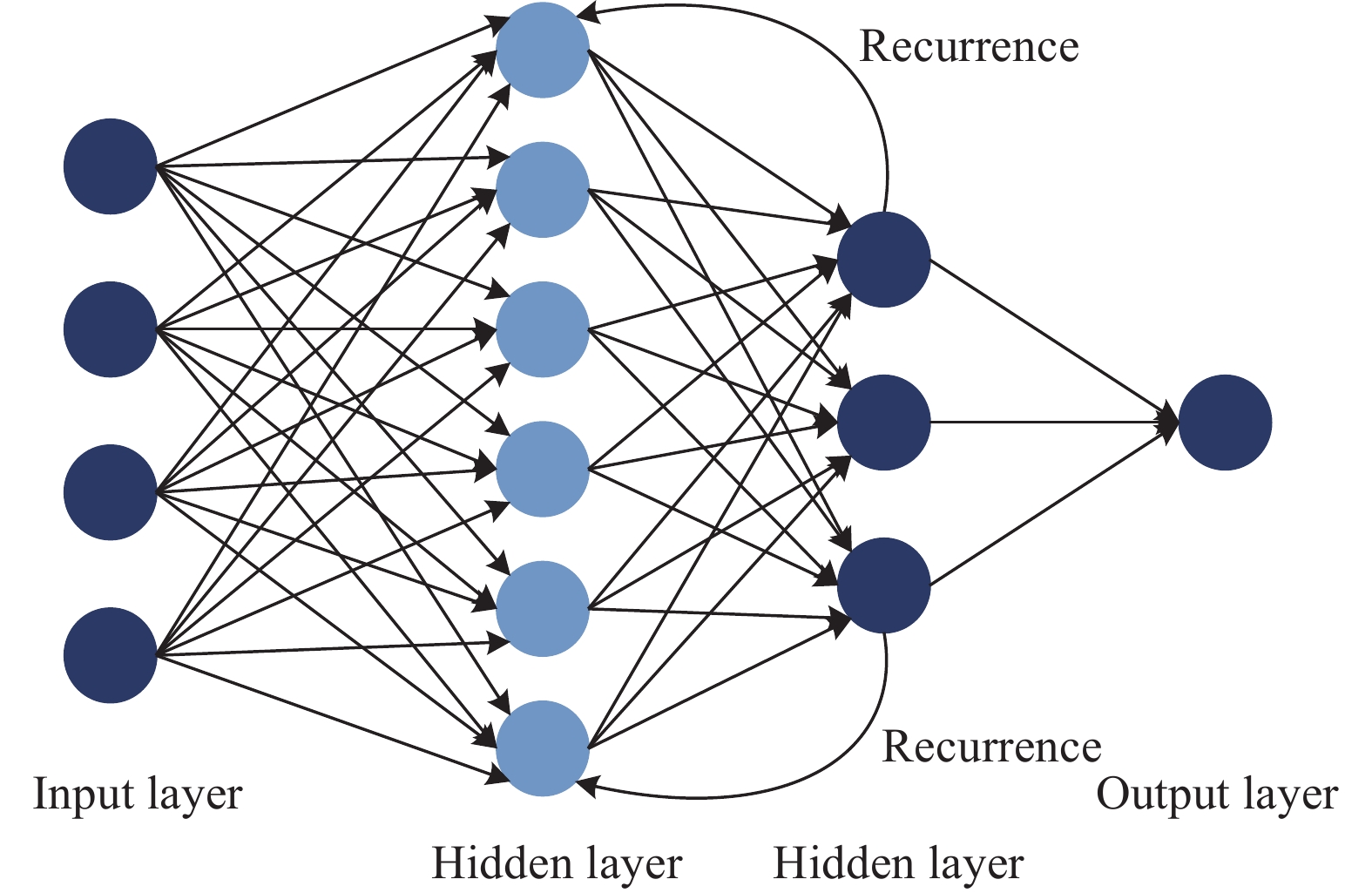
A RNN extends the traditional feedforward neural network, which can predict the input sequence data. It learns the hidden representation of the variable length input sequence through the internal recurrent hidden variables; the output of the activation function of the hidden variables at each moment depends on the output of the activation function of the recurrent hidden variables at the previous moment^[34], which can use the information of the previous moment, so the RNN has the function of memory. Fig. 4 illustrates the simple architecture of the RNN.

Figure  4.  RNN infrastructure.

下载: 全尺寸图片 幻灯片

There are various types of RNNs, including long and short-term memory networks, gated recurrent unit networks, and deep RNNs. RNNs are usually learned using backpropagation algorithms, and their application areas include natural language processing, speech processing, and time series prediction.

2.2.4   Transformer Model

The transformer model is a DL model based on the self-attention mechanism^[35] and consists of two parts, the encoder and the decoder, each consisting of several identical sublayers stacked on top of each other. Each sublayer of the encoder mainly consists of a multi-head self-attention mechanism and a feedforward fully-connected network, which generates a weighted contextual representation by calculating the attentional weights between different positions in the input sequence and a feedforward fully-connected network that performs independent nonlinear variations of the representation at each position. Each sublayer usually consists of two fully-connected layers and an activation function. Each sublayer is followed by a residual connection, and layer normalization is used to accelerate training and stabilize the network. Each sublayer of the decoder consists of a multi-head self-attention mechanism, an encoder-decoder attention mechanism, and a feedforward fully-connected network, where the decoder generates a new target sequence based on the encoder's output. Because the Transformer model does not have a mechanism for sequential processing of sequences, it adds positional encoding to the input embedding to permit the use of sequential information from the input sequences. Initially used for natural language processing tasks, the Transformer model has been widely used in astronomy for processing various types of time sequences, spectral data, and image data.

As the core technology of artificial intelligence, ML has gradually become an important tool for solving astronomical data processing problems, given its powerful data processing and pattern recognition capabilities. Data classification and prediction can be conducted effectively through the statistical model in ML. Neural networks in DL, especially CNNs, have a strong adaptive ability to complex high-dimensional data. In astronomical data processing, the application of these techniques is able to not only improve the efficiency and accuracy of data processing but also provide more possibilities for exploring the hidden scientific laws of the universe. Table 2 summarizes the commonly used models and their applications of ML in astronomy in recent years^[36–38].

Table  2.  Standard models and applications of ML in astronomy

	Standard learning methods/models	Application in astronomy
Traditional ML	Supervised learning methods: perceptual machines, kNN, Naive Bayes, logistic regression, SVMs, Boosting, decision trees, and random forests (RF)	Classification of astronomical spectra[39], Classification of active galactic nuclei[40], Classification of supernovae[41], Identification of single pulses[42], Radio-frequency interference suppression[43], Search for fast radio bursts[44], Identification of pulsar candidates[45], Classification of galactic spectra[46]
	Unsupervised learning methods: clustering methods, SVD, PCA, Markov Chain Monte Carlo	Stellar spectral analysis[47], spectral cluster analysis[48], Stellar atmospheric parameter estimation[49], Hydrogen atom clock troubleshooting[50], Galaxy spectral classification[51], Pulsar candidate identification[52], RF interference suppression[43]
DL	Feedforward neural networks	Galaxy photometric redshift estimation[53], Gamma-ray burst identification[54], Feeder compartment fusion measurement prediction[55], Stellar atmosphere parameter estimation[56]
	CNNs	Galaxy morphology classification[57], Star formation rate measurements[58], Spectral redshift estimation[59], Cosmological parameter estimation[60], Merging galaxy clusters identification[61], Galactic photometric redshift prediction[62], Coronal ejecta detection[63], Pulsar candidate identification[64], Fast radio burst classification[65], Radio-frequency interference detection[66], Gravitational wave signal detection[67], Stellar spectral classification [31], Stellar atmospheric parameter prediction[68], Fast radio burst search[69], Galaxy spectral classification[70]
	RNNs	Global 21-cm spectral line signal simulation[71], RF interference detection[72], Supernova classification[73], Strong gravitational lens parameter prediction[74], Variable star classification[75], Pulsar candidate identification[52], Stellar atmosphere parameter prediction [76], Stellar spectral classification[77]
	Generating adversarial networks	Stellar spectral classification[78], Pulsar candidate identification[79]
	Autoencoder	Gamma-ray burst identification[80], Galaxy image compression and denoising[80], Stellar spectral classification[81], Defective spectral recovery[81]
	Transformer model	Gravitational wave signal detection[82], Stellar spectral classification[83], Galaxy morphology classification[84], Photometric redshift estimation[84], Stellar atmospheric parameter prediction[85], Stellar spectral restoration [85]

下载: 导出CSV 

| 显示表格

3.   APPLICATION OF ML TO SPECTRAL DATA PROCESSING

3.1   Measurements of Stellar Atmospheric Parameters

Measurement of stellar atmospheric physical parameters, including stellar surface effective temperature T_eff, surface gravity log g, metal abundance [Fe/H], and microscopic turbulent velocity, helps to model stars of different masses, ages, and evolutionary stages. As an important unit of galaxies, the study of the physical parameters of a large number of stellar atmospheres in galaxies can reveal the evolutionary process of galaxies. There are direct and indirect measurement methods for stellar parameters, and indirect measurement methods are the primary means of stellar atmospheric measurements at present, including photometric methods, infrared flux methods, Balmer line profile fitting, and spectral template fitting^[86]. With the arrival of the astronomical big data era and the rapid development of ML algorithms, data-driven stellar atmospheric parameter measurement methods based on combining ML algorithms and spectra with large data volumes are the current major trends.

Stellar spectral data are complex and nonlinear, with intricate relationships between spectra and physical parameters. Extracting comprehensive information and understanding the relationships between these parameters are major challenges in spectral data mining^[87]. With the prominence of ML in modeling nonlinear relationships, more studies have adopted ML methods to predict stellar spectral parameters. Stellar spectral parameter estimation using traditional ML methods usually includes two processes: spectral feature extraction and mapping learning. Zhang et al.^[88] designed the stellar labeler SLAM based on the support vector regression technique for extracting the stellar parameters from an extensive survey spectral dataset. The SLAM model uses the cross-validation data of LAMOST DR5 and APOGEE DR15. Eight-fold cross-validation is used during training to find the best-fitting hyperparameters. The SLAM model predicts poorly for low signal-to-noise data, and the computational cost and storage requirements increase significantly as the number of labels in the training set increases. Xiang et al.^[89] have used PCA for feature extraction by mapping spectra to feature space using a nonlinear function. Model training and testing revealed that the prediction results for spectral data with R_SN ≥ 50 were better than those for low SNR data.

Traditional ML methods rely on labeled data and have poor prediction results for low Signal-to-Noise Ratio (SNR) data. With the increase in data volume and the development of DL methods, artificial neural networks have been applied to predict atmospheric parameters of stellar spectra. Li et al.^[90] proposed the StarGRUNet model based on artificial neural networks and self-attentive learning mechanisms. 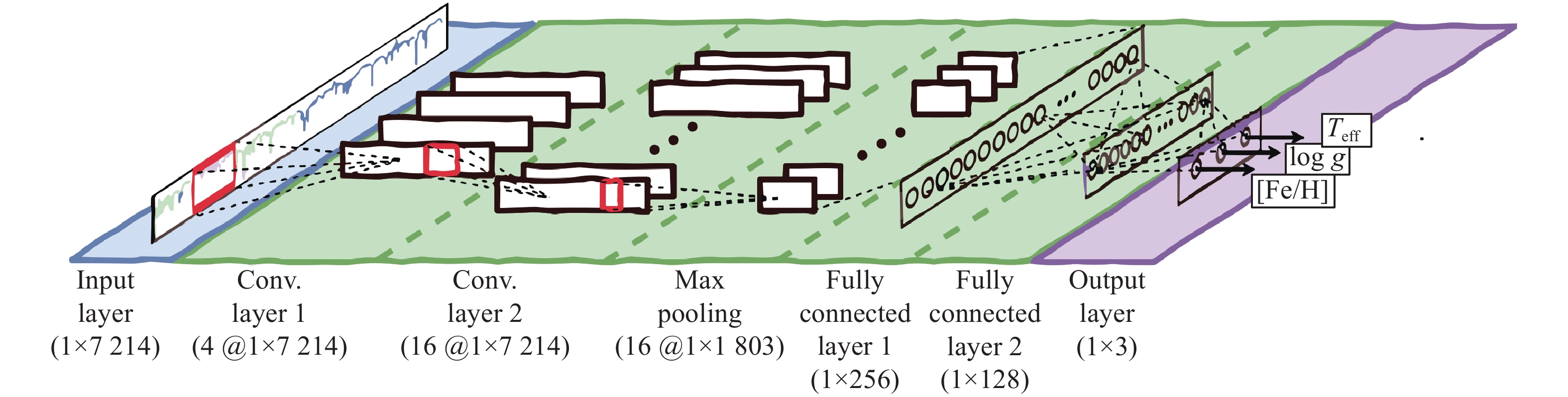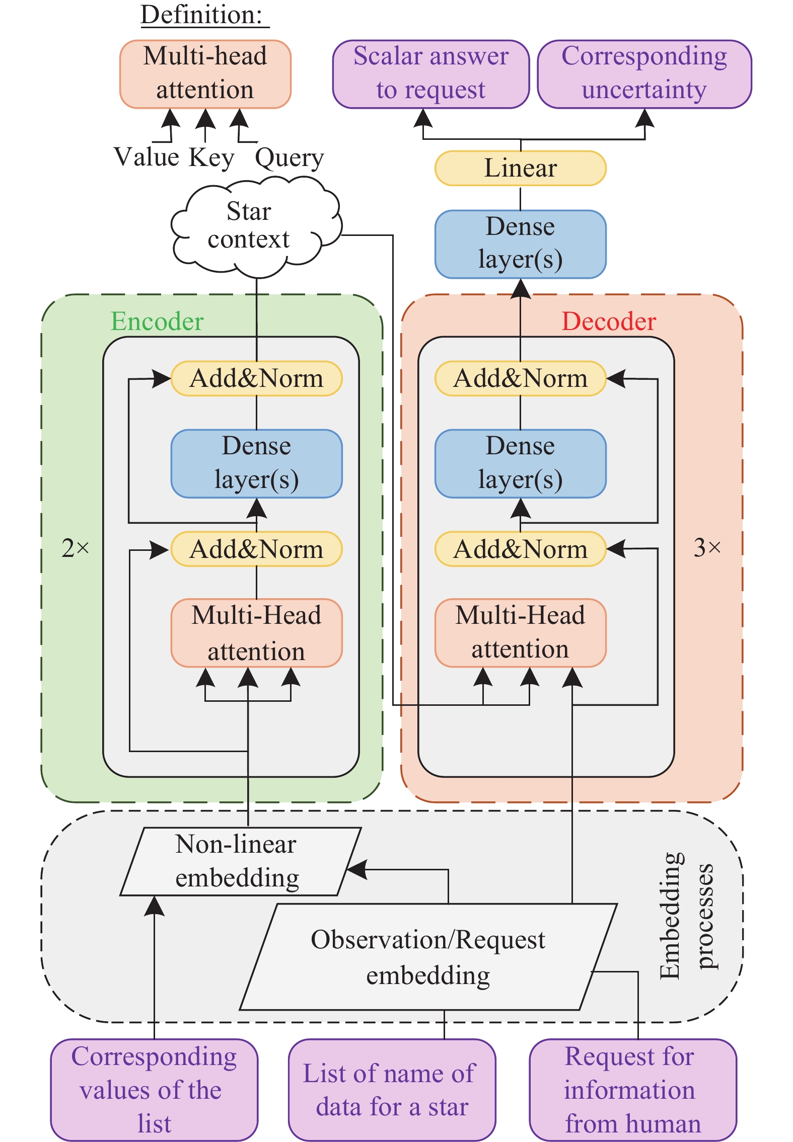The self-attentive module was used to learn different types of spectral parameter features; the model uses data with 5 ≤ R_SN ≤ 50 and R_SN ≥ 50, the test set contains 67340 and 100973 entries each, and the test set contains 19240 and 28850 entries each. The model test results reveal that for spectral data with signal-to-noise ratios greater than or equal to 5, the prediction accuracies of StarGRUNet for T_eff and log g are 94 K and 0.16 dex. Li et al.^[91] constructed a deep CNN based on the open-source python package of astrNN to predict the abundance of nine elements in stellar spectra simultaneously, and to avoid the prediction error caused by the uneven distribution of the sample set, the researcher added a weight matrix to the loss function. Pan et al.^[56] used feedforward neural networks for stellar atmospheric parameter prediction, using 50000 spectral data released by SDSS, with training and test sets of 5000 and 45000 spectra. The results of the study indicated that the mean absolute errors for the effective temperature T_eff, surface gravity log g, and metal abundance [Fe/H], were respectively 79.95 K, 0.1706 dex, and 0.1294 dex, and the model uses stacked self-coding neural network to effectively overcome the problems of local minima and gradient dispersion in the training process of traditional backpropagation neural network. Wang et al.^[92] proposed a stellar atmospheric parameter measurement algorithm combining CNNs and RF, using CNNs to extract features from pseudo-two-dimensional images generated based on the spectra, extracting higher-dimensional nonlinear features in the spectral data, and improving the prediction accuracy. Fabbro et al.^[68] applied a deep neural network architecture to analyze the stellar spectra, using the APOGEE stellar spectral dataset to train the CNN model StarNet. StarNet extracts the spectral line feature information in the spectra by window splitting to predict the star’s effective temperature, surface gravity, metal abundance, and other parameters. The StarNet model architecture is depicted in Fig. 5. The initial training of the model uses the APOGEE ASSET grid to generate 300000 synthetic spectral data, of which 224000 were used as the training set, 36000 as the validation set, and 40 000 as the test set. The StarNet model and Cannon2 model^[93] were used for training and testing on 85341 spectra of the APOGEE DR12 dataset. The models were evaluated using mean absolute error (MAE) and root mean square error (RMSE) as the evaluation metrics for prediction performance. The StarNet model had superior prediction ability, as presented in Table 3. The StarNet model has superior prediction ability on high SNR spectra, which is consistent with the ASPCAP data processing standard pipeline. However, the prediction error is larger in low signal-to-noise spectra. The test reveals that the differences in the size of the training set samples, the range of stellar parameters, and the training time can cause differences in the training results.

Figure  5.  Architecture of 7-layer StarNet model based on CNN^[68].

下载: 全尺寸图片 幻灯片

Table  3.  StarNetc2 model and Cannon2 model APOGEE DR12 data test results^[68]

Model	Metric	Teff/K	log g/dex	[Fe/H]/dex
StarNetc2	MAE	31.2	0.053	0.025
	RMSE	51.2	0.081	0.040
Cannon2	MAE	46.8	0.066	0.036
	RMSE	71.6	0.102	0.053

下载: 导出CSV 

| 显示表格

Aiming to solve the problem of noise interference during stellar spectral feature extraction, Xiong et al.^[94] proposed the residual RNN RRNet, which is used primarily for estimating stellar parameters from LAMOST medium-resolution spectra. RRNet mainly consists of residual, recurrent, and uncertainty modules and suppresses the effects of noise and irrelevant components by enhancing the spectral features. The model performance improves with the increase of hyperparameters, but when the hyperparameters reach a certain threshold, the performance improvement is weak or even decreases. Adding more residual blocks can help improve the ability to extract spectral information. However, the training set cannot be infinitely scaled to support higher complexity models in practical applications. Leung et al.^[85] trained a stellar astronomical model based on the Transformer and large-scale language modeling techniques, as well as a stellar astronomical base model. Fig. 6 illustrates the model's architecture, which performs generative and discriminative tasks, including implementing stellar parameter extraction, spectral generation and restoration, and mapping between stellar parameters. The model was trained by a self-supervised learning approach using data such as APOGEE and Gaia. In the task of mapping from spectra to stellar parameters, the model's prediction accuracies for the T_eff, log g, and [M/H] parameters are 47 K, 0.11 dex, and 0.07 dex, which illustrate comparable accuracies to that of the fine-tuned XGBoost model. The model can handle multiple tasks without fine-tuning and provide prediction inaccuracy, making it competitive with traditional machine learning models.

Figure  6.  Neural network architecture of the transformer-based stellar astronomical base model^[85].

下载: 全尺寸图片 幻灯片

3.2   Classification of Stellar Spectra

Traditional spectral classification methods usually rely on researchers comparing spectra with standard stellar samples by the naked eye^[95], which, despite its pattern recognition and classification capabilities, is inherently subjective, and the process of visual inspection through the human eye is highly time-consuming and difficult to handle large amounts of data. With the increasing volume and complexity of astronomical data, traditional spectral classification methods are becoming obsolete, and the solution to these problems is the development of automated methods based on the quantitative determination of spectral features. von Hippel et al.^[96] proposed a pattern recognition-based approach to achieve spectral classification by mimicking the operations of a human classifier when visually inspecting spectra and estimating their presence. Scibelli et al.^[97] achieved spectral recognition based on searching for spectra that are most similar to the observed spectra in a library of template spectra of different spectral models, correlating the observed spectra with the spectra in the template spectral library, and classifying to which class of spectra they belong based on the magnitude of their correlation coefficients. These automated techniques are an improvement over naked-eye classification. However, they are difficult to apply to spectral data of different resolutions generated by different observing instruments and observing modes, and the pattern-matching method suffers from low efficiency and few standard star spectra.

With the deepening of machine learning research and applications, more machine learning methods are used to analyze and process astronomical spectral data. Liu et al.^[98] applied SVMs to the classification of stellar spectra and found that the completeness of classification was as high as 90% for A- and G-type stars, but for O-, B-, and K-type stars, the completeness was as low as 50%, resulting in about 40% of the O-, B-, and K-type stars being respectively were misclassified as A- and G-type stars. Thus, traditional machine learning methods are prone to large errors when facing multi-class classification tasks, especially when the classes are unbalanced. Zhang et al.^[99] establish a stellar spectral classification model based on multi-class SVMs, which solves the problem of higher complexity of SVMs when targeting multi-classification problems. However, model prediction accuracy is not high. Zhang et al.^[100] propose the XGBoost-based stellar spectral feature classification method that uses the XGBoost algorithm (for automatic classification and feature ranking) to obtain the known or unknown spectral lines most sensitive to the classification decision.

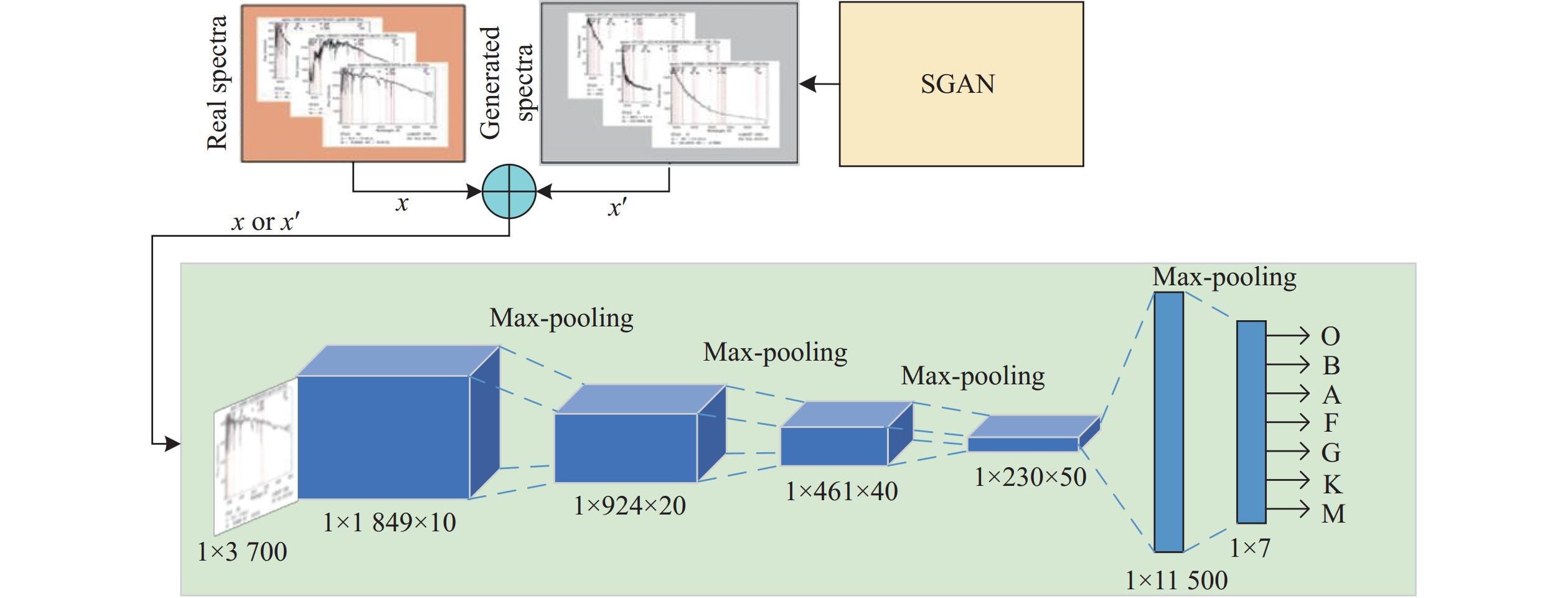
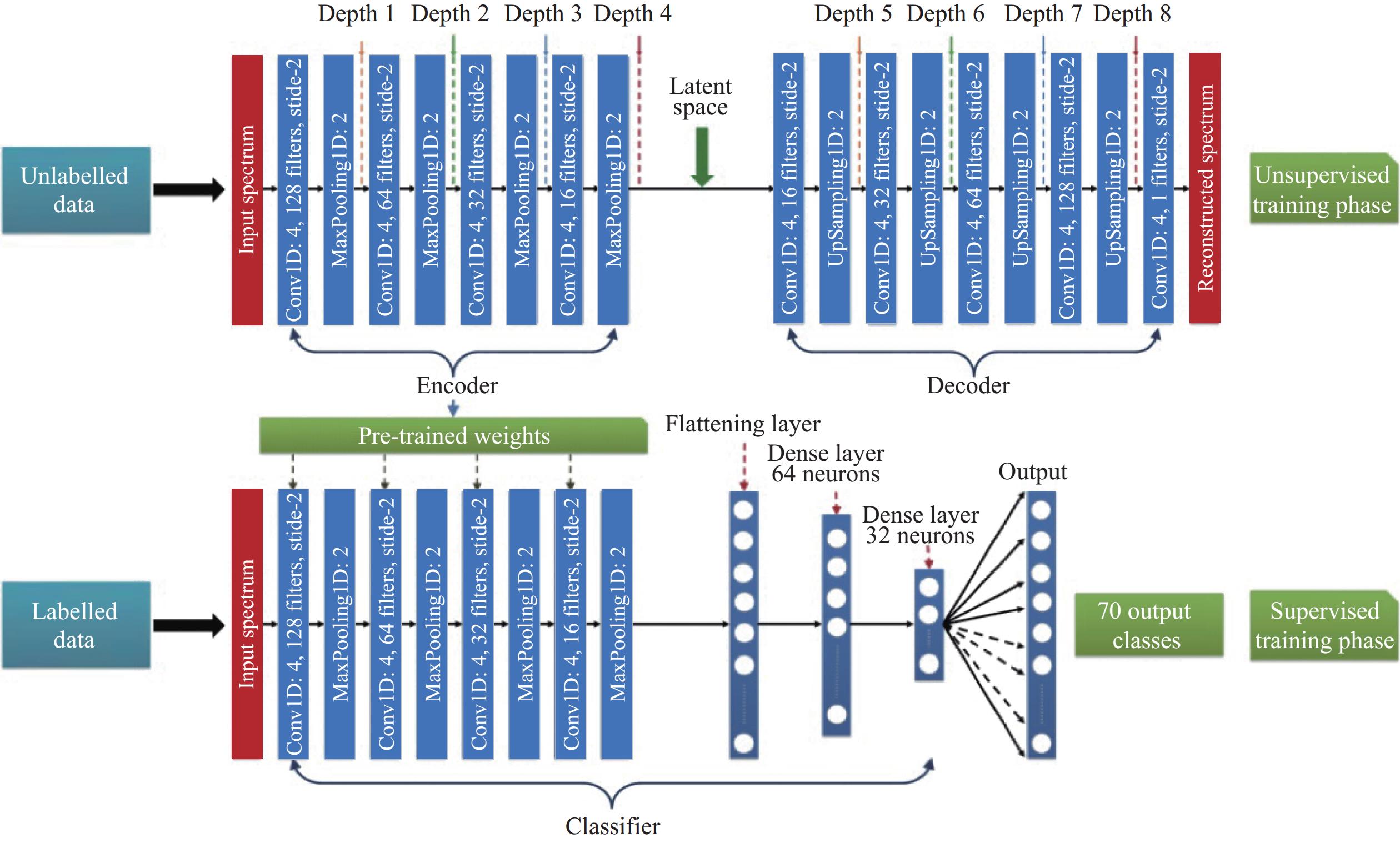
Traditional machine learning algorithms can extract several layers of stellar spectral features, cannot extract high-level features, and are susceptible to the imbalance of the training set, and therefore DL methods have been gradually applied to the stellar spectral classification problem. Zheng et al.^[101] proposed a spectral generation method based on a one-dimensional generative adversarial network used to balance the training sample dataset, and then a CNN was used for the classification task. The model architecture is depicted in Fig. 7, and the model is used for O-, B-, A-, F-, G-, K-, and M-type star classification, and the average correct rate of classification is 95.3%. Liu et al.^[102] proposed a supervised algorithm for stellar spectral classification on the basis of one-dimensional stellar spectral CNN to classify F-, G-, and K-type stellar spectra and their subclasses and compared the model with the Artificial Neural Network Algorithms, random forest algorithms, and SVM algorithms. The one-dimensional CNN model has the highest classification accuracy on the same dataset. Hong et al.^[103] used CNN to extract the deep features of spectra and combine them with the attention mechanism to learn the important spectral features. It reduced the spectral dimensions by pooling operations to compress the number of model parameters. The method achieved an accuracy of 92.04% in the classification of F-, G-, and K-type stellar spectra. Wang et al.^[81] developed a deep neural network-based automatic astronomical spectral feature extraction method applied to astronomical spectral classification and defective spectral repair. The method uses a pseudo-inverse learning algorithm to train a multilayer neural network layer by layer to automatically extract features from spectral data. It uses a softmax regression model for classification. 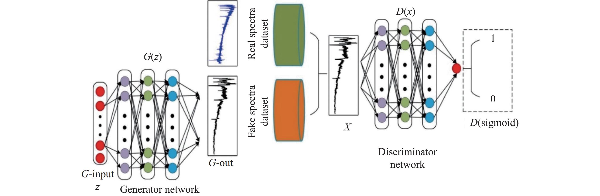When the number of training samples is 608483, and the number of networks in the model is increased to 12, the model has F₁ scores of 0.8549, 0.7891, and 0.8499 for the classification of F-, G-, and K-type stars. Sharma et al.^[104] proposed to use a CNN model for the automatic classification of stellar spectra with the model architecture depicted in Fig. 8, which uses an autoencoder for pre-training of unlabeled spectral data, adjusting the weights of the encoding and decoding layers, and then supervised training based on the labeled data.

Figure  7.  Combined CNN and SGAN architecture^[101].

下载: 全尺寸图片 幻灯片

Figure  8.  Semi-supervised one-dimensional CNN classification model architecture^[104].

下载: 全尺寸图片 幻灯片

On the basis of the remarkable progress of CNNs in astronomical spectral classification, researchers have proposed several improved models to increase classification accuracy and processing efficiency. Liu et al.^[105] proposed a hybrid DL network BERT-CNN combining Transformer and CNN, which captures the intrinsic relationship between spectral features through the self-attention mechanism in Transformer, compresses the features through the pooling layer in the CNN, and finally integrates the features through the all-connectivity layer and outputs the classification results through a softmax classifier. Han et al.^[106] proposed a stellar spectral classification model MSFnet based on multiscale feature fusion, using the multiscale fusion module to preprocess the data and inputting the processed data into a four-layer CNN model for the classification task, and successfully classified the stellar spectra into the six types of B-, A-, F-, G-, K-, and M-type. Zou et al.^[107] proposed a convolutional network that combines the residual mechanism and attention mechanism for astronomical spectral classification, using convolutional operations to extract shallow and deep features into the spectral data, the residual mechanism to increase the depth of the network, and the attention mechanism to enable the network to focus on specific spectral bands and features to make the learning process more targeted. Liu et al.^[78] proposed StellarGAN, a stellar spectral classification model based on GANs, and the training process of the model is depicted in Fig. 9; in the pre-training stage, the model is trained using unlabeled stellar spectra and spectra generated by generative networks, and the fine-tuning phase is retrained using labeled spectra. The StellarGAN model was trained with SVM, RF, PCA, LLE, and CNN using the same number of training and test sets, where the StellarGAN model obtained the highest F₁ score (0.63) on the SDSS dataset using only 1% of the labeled data, compared with SVM, RF, CNN and other traditional methods, StellarGAN has a clear advantage in small sample learning. The experimental results also reveal a direct relationship between the spectral signal-to-noise ratio and the F₁ score. When the signal-to-noise ratio is low, the F₁ score also decreases.

Figure  9.  Schematic of the StellarGAN model training process^[78].

下载: 全尺寸图片 幻灯片

4.   CONCLUSIONS

This paper systematically analyzes the application of machine learning methods in stellar spectral atmospheric parameter prediction and stellar spectral classification, where Table 4 summarises the test results of the relevant literature in the task of predicting stellar spectral atmospheric parameters, and Table 5 shows the test results of the relevant literature in the task of classifying stellar spectral. In the stellar spectral atmospheric parameter prediction task, CNN and Transformer models perform the best in prediction. Although the CNN model performs well on small-scale data, Transformer is more advantageous for large-scale data. However, the performance of all the models is degraded on low signal-to-noise spectral data, and the computational cost and storage requirements increase significantly with large-scale datasets. For stellar spectral classification, CNNs far outperform traditional machine learning methods. Generative multi-resistance network methods achieve better classification results by combining a large amount of unlabeled data while relying on a small amount of labeled data, and cross-modal models based on the Transformer method can achieve the same level of classification ability as supervised learning models while achieving multi-classification. Transformer-based cross-modal models can realize multi-class tasks while achieving the same classification ability as supervised learning models.

Table  4.  Literature test results related to the application of ML in the prediction of stellar spectral atmospheric parameters

	Model	Training set	Test set	Indicators	Teff/K	log g/dex	[Fe/H]/dex	[M/H]/dex
Zhang et al.[88]	SVR	17175	8171443	Prediction error	49	0.10	—	0.037
Li et al.[90]	Artificial Neural Networks(ANNs)	168313	48090	MAE	49.28	0.084	0.041	—
Li et al.[91]	CNNs	68363	7596	MAE	29	0.07	0.03	—
Pan et al.[56]	FNNs	5000	45000	MAE	79.95	0.1706	0.1294	—
Fabbro et al.[68]	CNNs	12681	85341	MAE	31.2	0.053	0.025	—
Xiong et al.[94]	RNNs	80812	23198	MAE	51.7068	0.0808	0.0308	—
Leung et al.[85]	Transformer	397718	44080	Prediction error	47	0.11	—	0.07

下载: 导出CSV 

| 显示表格

Table  5.  Literature test results related to the application of machine learning on the classification of stellar spectra

	Model	Spectral type	Training set	Test set	Accuracy	Precision	Recall	Harmonic mean F1
Zhang et al.[100]	XGBoost	F	840375	280125	0.8988	—	—	—
		G	1507318	502440	0.8537	—	—	—
		K	357752	119251	0.9234	—	—	—
Zhang et al.[100]	GAN CNNs	F	1000	400	0.958	—	—	—
		G	1000	400	0.960	—	—	—
		K	1000	400	0.975	—	—	—
Wang et al.[81]	DNNs	F	12994	2293	—	—	—	0.8468
		G	16448	2903	—	—	—	0.7747
		K	13058	2304	—	—	—	0.8427
Sharma et al.[104]	CNNs	F	155	27	—	0.92	0.98	0.95
		G	251	44	—	0.89	0.89	0.89
		K	221	39	—	0.88	0.89	0.89
Liu et al.[105]	Transformer CNNs	F	3585	1536	0.9108	0.9565	0.9708	0.9656
		G	1779	762	0.9239	0.9620	0.9659	0.9639
		K	2269	972	0.9311	0.9696	0.9809	0.9752
Han et al.[106]	CNNs	F	5762	1921	0.951	0.961	0.952	0.956
		G	5763	1922	0.957	0.96	0.953	0.956
		K	5766	1922	0.975	0.957	0.975	0.966

下载: 导出CSV 

| 显示表格

Artificial intelligence techniques still have limitations when performing astronomical spectral analysis tasks. In the classification problem, the uneven distribution of training sample data and low spectral signal-to-noise ratio affect the model performance, and part of the model performance relies on a large amount of high-quality labeled data, which requires human resources and time for noise reduction and labeling. This requirement is because astronomical data processing involves a complex physical background, the ''black-box'' characteristic of the model makes it difficult to generate an explanation, the consumption of computational resources is significant, and model training and reasoning require a large amount of computational resources.

Future advancements could focus on developing data augmentation techniques to create high-quality simulated datasets using generative adversarial networks. Additionally, DL approaches that remove the need for manual feature extraction from raw data could be explored, along with the adoption of semi-supervised or unsupervised learning methods. These approaches would enable the use of novel structures within unlabeled data, expanding training datasets or creating standardized datasets.

Furthermore, the development of interpretable models capable of providing scientifically meaningful insights should be prioritized. Establishing foundational models of astronomical phenomena and training generalized models using large-scale survey and multi-band astronomical datasets could significantly reduce the time needed for iterative model training and inference. With the development of computer hardware and software technology and the improvement of artificial intelligence algorithms, the combination of artificial intelligence and astronomy is an inevitable trend in the development of astronomy. Artificial intelligence-related technology can provide astronomical data analysis with higher processing efficiency of spectral line data, realize seamless docking and comprehensive analysis of multi-source data, and provide richer, multidimensional information support for the comprehensive revelation of the mysteries of the universe.